Basic workflow
Knowing the tools in Photoshop is one thing, but applying them in a sensible and logical order that will enable a repeatable approach to each photograph, not simply by following a list of instructions, but by analysing the photograph and planning a logical work order is quite another. Start with the (optional) importation of the RAW file, or the simple opening of the JPEG, then move on to layers and selections to the final result.
OPENING RAW FILES
Lightroom is excellent for storing, cataloguing and cross-referencing files – so you can simply open files directly into Photoshop from Lightroom.
Opening a RAW file directly into Photoshop requires the use of a RAW converter – usually Adobe Camera RAW, within Preferences>File handling, one of the tick boxes we didn’t alter was ‘Prefer Adobe Camera RAW for supported RAW files’.
Either click on File>Open, or use the shortcut Ctrl-O, or simply double-click in the grey area in the middle of the screen and you get the open dialogue box. Select an appropriate file to open – with RAW files, all you see is the file logo – NEF for Nikon, CR2 for Canon, ORF for Olympus and so on. Not as helpful as it might be – though most people who don’t use Lightroom use Adobe Bridge, which will allow you to view the file picture.
The Adobe Camera RAW box will appear with the picture within it.
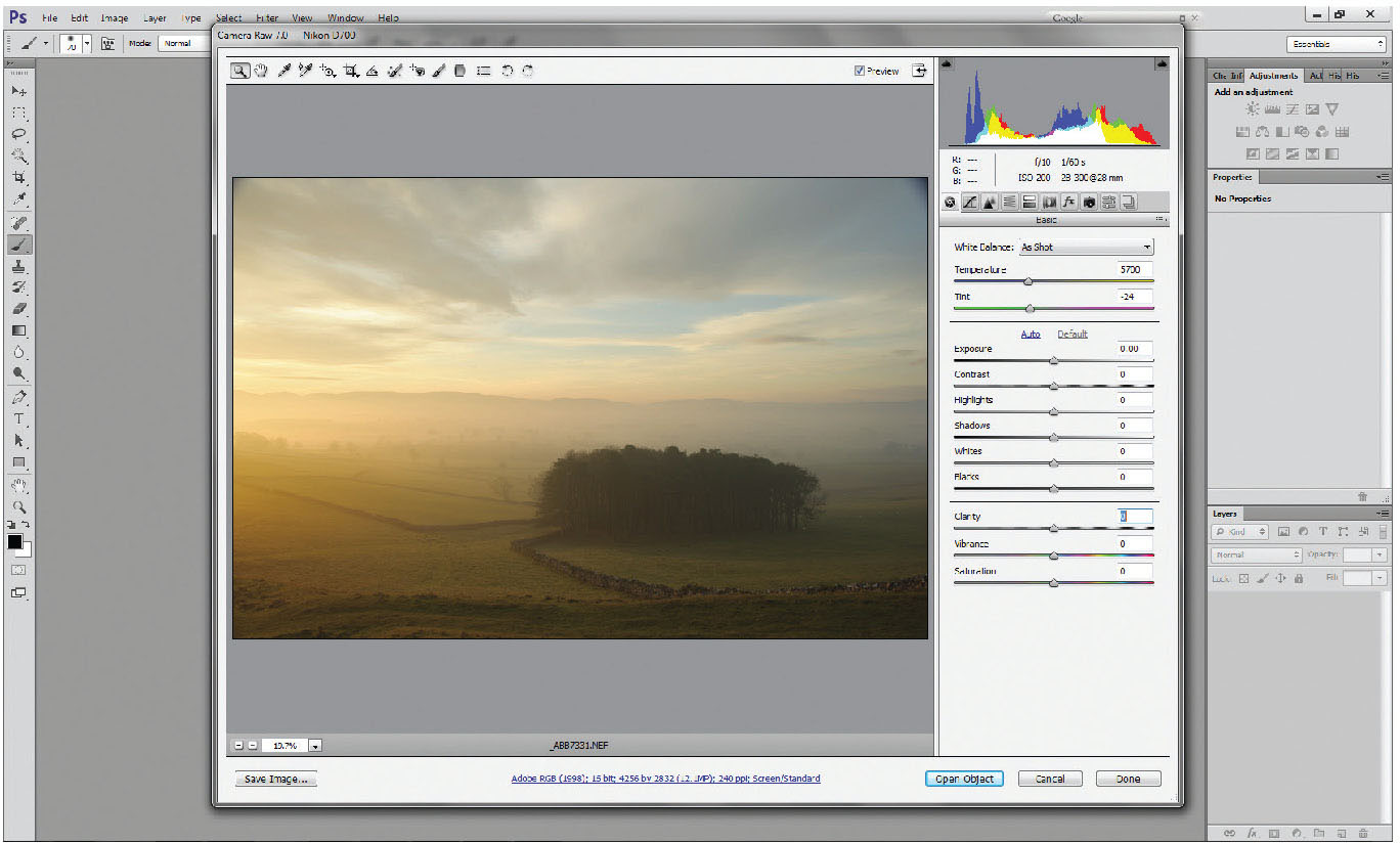
Fig. 4.1
Adobe Camera RAW with all sliders set to 0 (default) showing unadjusted RAW file.
As you see, all the sliders on the right of the panel are set to 0 as the Photoshop default. Many users like to do as much work in Camera RAW as possible. Remember that adjustments made on separate adjustment layers can be reviewed and re-edited, whereas adjustments to the RAW image cannot be altered apart from reopening the RAW file. For that reason, do relatively little work in Camera RAW – just making those changes that either cannot easily be made in Photoshop or that will make it easier to use Photoshop.

Fig. 4.2
Adobe Camera RAW converter with alterations made to shadows and clarity in order to improve shadow detail and improve the textures (clarity) in the image.
In this example, the shadows in the copse of trees look a touch heavy – so by moving the ‘shadow’ slider to the right, it lifts the brightness of the shadow areas in the photo. The clarity slider is unique to Camera RAW, and may best be described as ‘micro-contrast’. Whereas simple ‘contrast’ lightens anything brighter than mid-grey, anything darker than mid-grey will become darker; clarity will – in this example – increase the contrast within the light sky area, whilst simultaneously increasing the contrast across the mid-toned grasses and even the darker copse of trees. As there is no equivalent filter within Photoshop, you could add a fair bit of clarity, as the original file was taken under pretty hazy conditions and just needed picking up a bit.
Camera RAW, with added clarity and boosted shadows.
That gets the file open, and into Photoshop, as a 16-bit ProPhoto RGB file with the basics done.
The next thing to do – and you should do this with every picture – is look closely at the photo. So many people don’t, and just press on with ‘processing’. In darkroom days, this is the time you would draw a printing plan – detailing the areas that would need lightening, and those that would need darkening. Digitally, it’s no different; look at the picture in a similar way, but also mentally consider areas that might need contrast enhancement as well (which was never possible printing colour in the darkroom).
Firstly, look for those little bits that most people overlook that need ‘tidying up’ – not major cloning, removing trees, adding sheep, or anything to change the nature of the photograph. No more than blemishes and the odd thing that we have no control over.
In the usual viewing mode, or by pressing Ctrl-0, the entire image fills the central area of the Photoshop screen, offering you as large a picture area as possible whilst still seeing the whole image. A typical high definition computer screen however has a resolution of 1920 × 1080 pixels (normal HD). The camera used for this picture (D700) has a resolution of 4256 × 2832 pixels, so to show them on a part of the 1920 × 1080 screen (remember the palettes, borders and so on that take up the outside of the screen) the picture has to be shown in a reduced size – in this case, the image is shown 31.4 per cent of its actual pixel size, meaning that each pixel on the screen is showing about 3 pixels in each direction of the actual picture.
By pressing Ctrl-1, zoom into 100 per cent magnification of the image – actual pixel size, where one pixel on the screen represents one pixel on the image. Almost always this will involve only seeing a very small part of the image on the screen at any one time. It does, however, show the sharpest possible image and reveal the greatest detail on the screen. You can navigate around the picture either by selecting the hand tool (H) or by simply holding the space bar down; the hand tool is temporarily invoked, enabling you to navigate around the screen, and by releasing the spacebar, you immediately return to your previously selected tool.
On this image there are a couple of sensor spots (never easy to keep 100 per cent clean) and a whole heap of tiny vapour trails in the sky to spoil the tranquillity. Getting rid of the spots is a necessity, the vapour trails is personal preference.
There are a number of ways all of this can be dealt with.
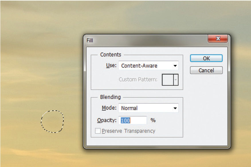
Fig. 4.3
Fill dialogue box set to use Content-aware fill, showing blending mode set to normal and 100% opacity (default settings).
Content-aware fill often works faultlessly, sometimes gets it tragically wrong. Tracing a ring around the spot with a lasso tool (or making a selection around it any other way) will leave a ring of marching ants. Hit the delete key and a small dialogue box appears.
The dialogue box should have ‘Content-aware’ under ‘Contents>use’. Hit enter and the spot will go, cloned effectively by sampling areas around the spot and interpolating brightness. The only thing questionable about content-aware fill is that it works directly on the background layer, and it’s often preferable to keep the background layer untouched.
An alternative way is to add a transparent (new) layer – it adds nothing to the file size and the best analogy is that it’s like laying a clear gel over an overhead projection slide. You can write on it, mark it, and it has no effect on the background layer. Using the spot healing brush tool (J) – make sure the right tool is selected, there are five options under the healing brush – Shift-J will let you scroll through the options. Make sure on the tool options at the top of the screen that the box to ‘sample all layers’ is ticked, and simply adjust the tool’s size (by using the square brackets) – the left bracket ([) makes the tool smaller, the right bracket (]) makes the tool larger – and simply click over the spot. On a subject like a dust spot, there will be no perceptible difference between content-aware fill or a healing brush. The covering to the spot sits on a separate layer (Layer 1) and you retain the ability to change or delete the repair right up until you flatten the image. It would be easy to remove the four vapour trails just below and to the left of the blue sky. Select them using a small brush in quick mask; on exiting quick mask, they simply become a marching ants selection, and with the background layer active, Delete>Enter performs a content-aware fill on the trails perfectly.
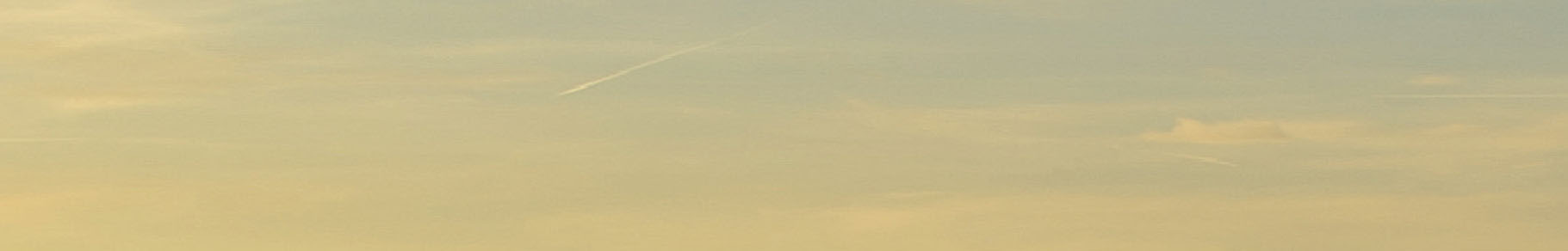
Fig. 4.4
Vapour trails visible within the sky.
Fig. 4.5
Quick mask/brush tool used to select trails quickly and easily.
Fig. 4.6
Repaired sky showing no visible vapour trails.
It’s important to perform cloning/repairs/content-aware fill at pixel size on the screen (100 per cent) as it lets you see as sharply as possible that your work is accurate.
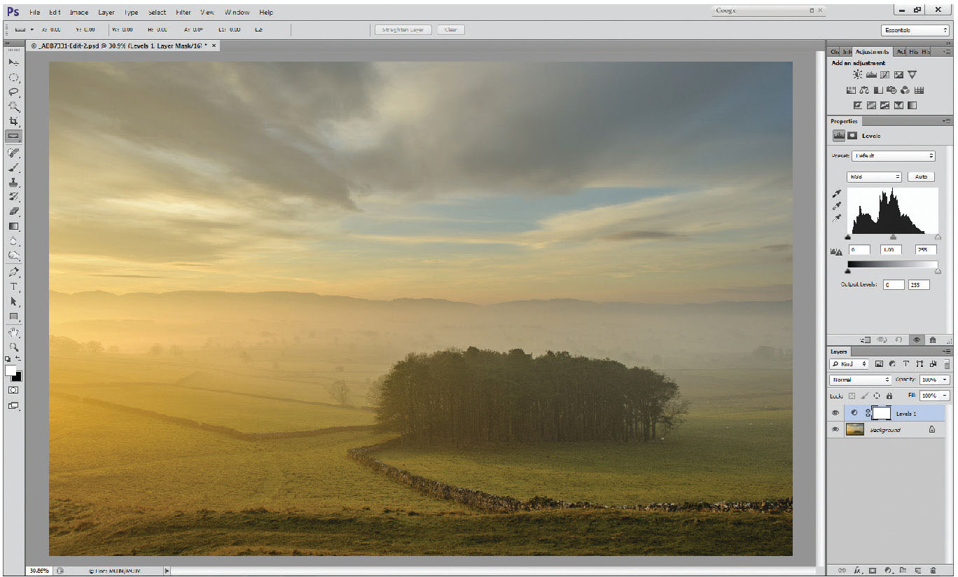
Fig. 4.7
Levels layer added above the background layer, no adjustment made yet.
Initially, take a good look at the histogram and the overall contrast range to see if a general levels layer is necessary.
By adding a levels layer you can see that the histogram falls short of the ends of the graph, suggesting that the image could take more contrast. (Effectively, the blacks could be darker, and the whites, whiter.)
On this image, it would be good to pull out a little more from the woodland so don’t change the dark tones yet, but instead just slightly brighten the highlights. On this image, the early morning tones are possibly slightly too warm. That can be adjusted at the same time.

Fig. 4.8
Highlights adjusted by moving the highlight slider from the right-hand end (value 255) to closer to the right end of the histogram (value 233) lightening the white values in the picture.
Firstly, slide the highlight slider to the left just to the edge of the histogram (Fig 4.8) – do not slide further than the end of the histogram, or you’ll clip highlight details. A good way of checking this is to hold down the Alt key as you move the highlight slider towards the histogram – as you depress the Alt key, the whole screen goes black, but as you pass the end of the histogram, those parts of the image that are being clipped show as bright tones. Just back the slider off until the screen is black, and you will have brightened the image as far as possible, whilst still retaining full highlight detail.
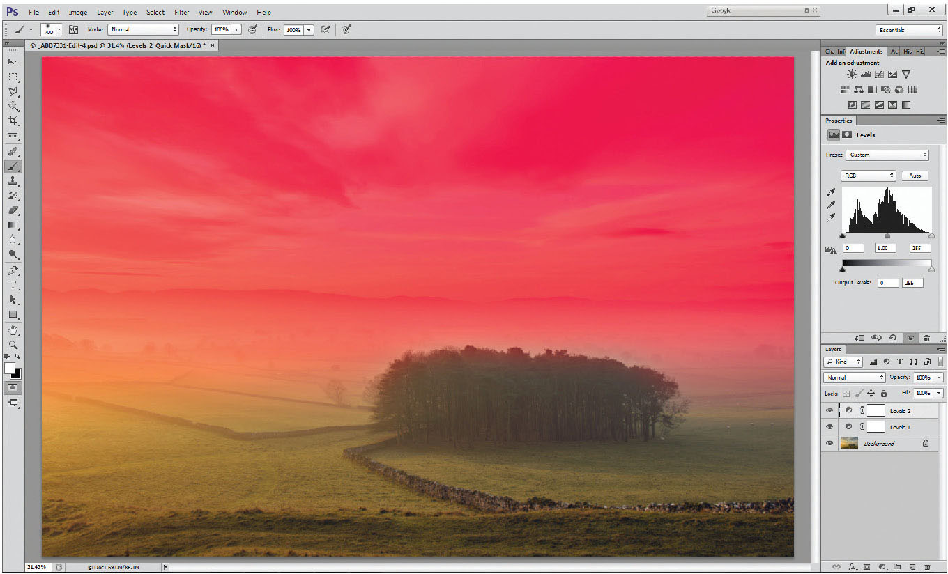
Fig. 4.9
Grey adjustment, set by using the mid-tone pipette to the left of the levels histogram, and clicking on a neutral grey tone within the image to set the white balance
The next stage is to correct the tones, which is a simple click if the picture has a neutral grey. Just to the left of the levels histogram are three pipettes – the top one black, the bottom white and the centre one grey. The top and bottom ones allow you to set a black or white point in the image (similar to moving in the end of the highlight/shadow sliders). The centre pipette allows you to select any point on the picture that should be a mid-grey. Click on the grey pipette and select part of the image that you see as a mid-grey – in this case, the distant hills on the extreme right of the picture. Click on that, and the colours right across the picture will change (Figure 4.9). If you clicked on a spot that changed the colours too far Ctrl-Z will undo the last action, and try again. Go on until you’re happy with the result.
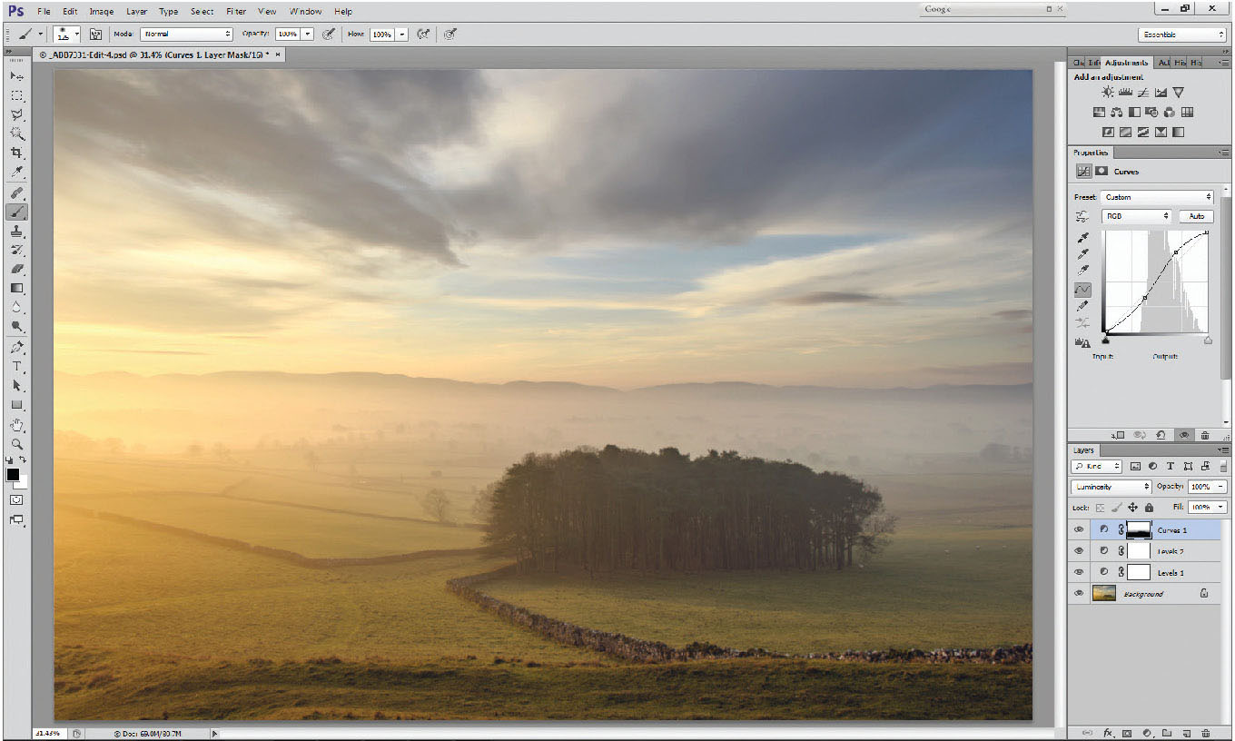
Fig. 4.10
Quick mask over sky by using the gradient tool (G) within quick mask (Q) to select the sky, with a soft edge at the horizon.
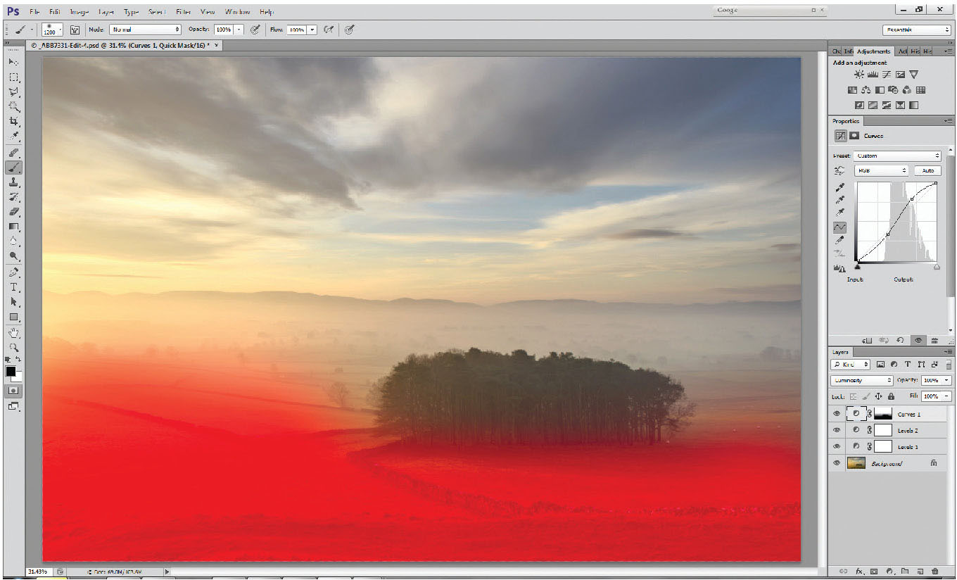
Fig. 4.11
Curves layer added to sky (AFTER exiting quick mask), increasing contrast to the sky tones.
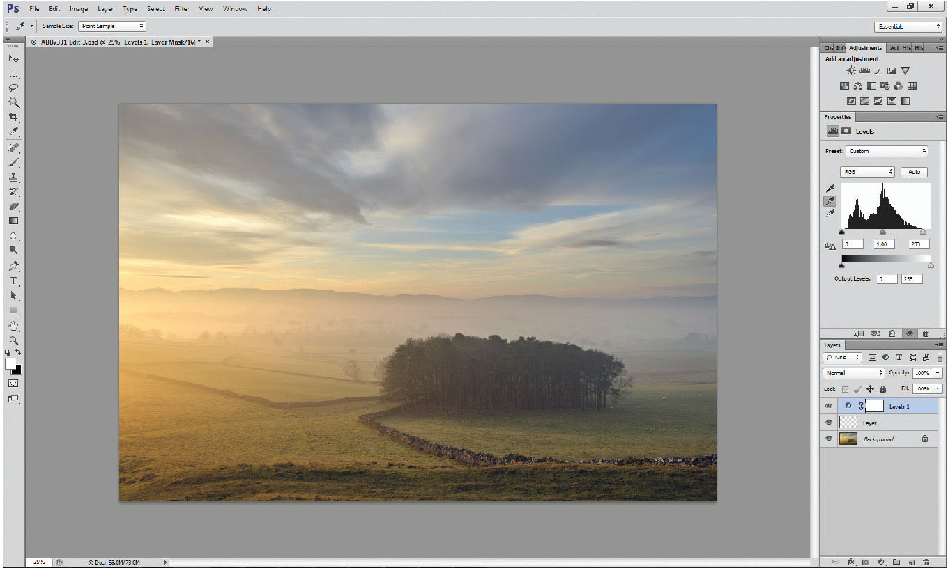
Fig. 4.12
Quick mask gradient selection added to foreground grass.
A sensible next step would be to add a touch more contrast to the sky – without adding any extra saturation. A quick mask (Q) and gradient tool (G) can select a good chunk of the sky, perhaps using a large white brush (B) (very soft edge) to exclude the area around the copse.
Exit quick mask (Q) to leave a selection, add a curves layer and add a touch more contrast to the sky – if you look at the histogram on the curves chart, you’ll see that by steepening it across the histogram that relates to the sky brightness, the contrast in the sky increases, making it stand out more in the picture.
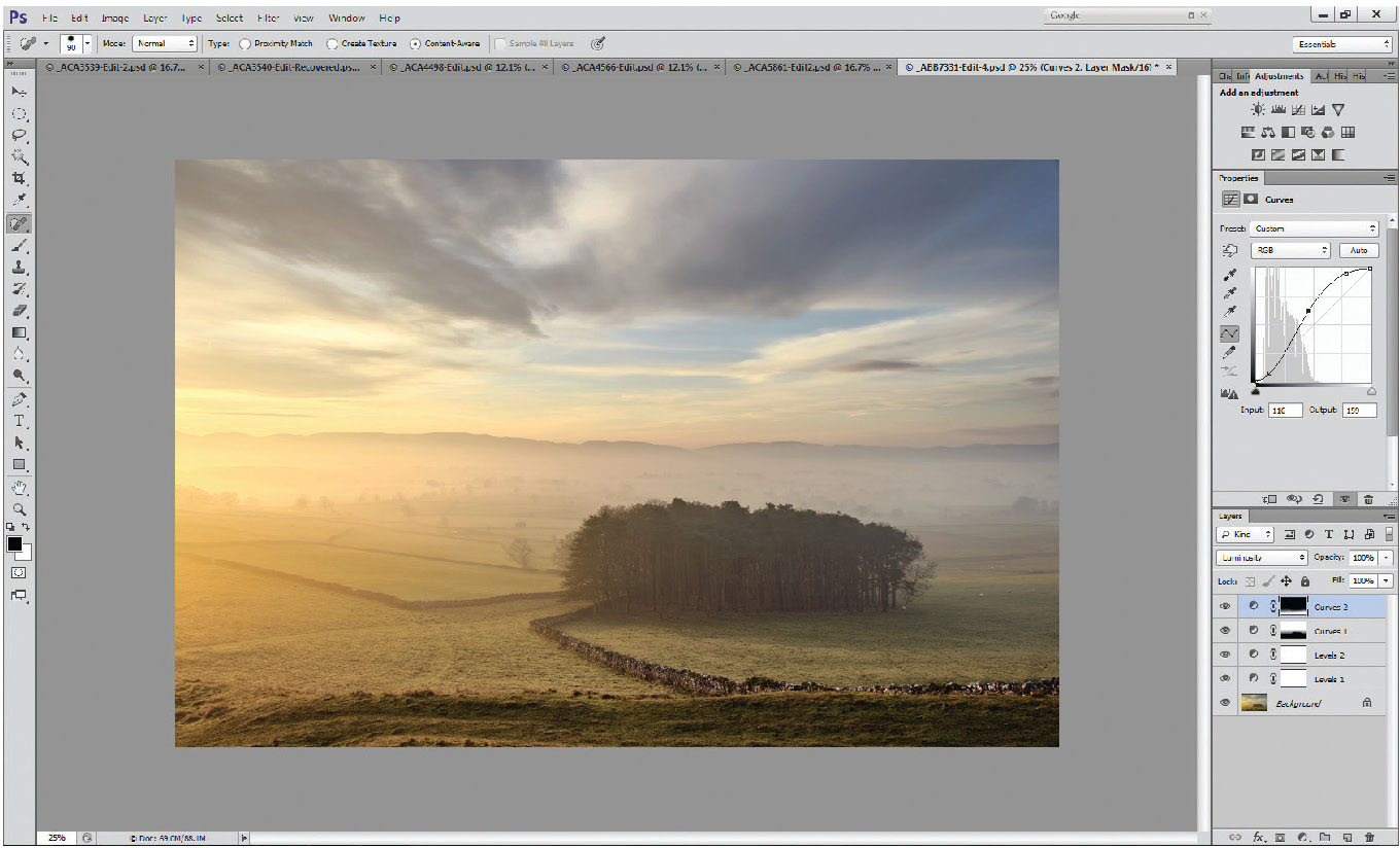
Fig. 4.13
Curves layer added to grasses to brighten the ground and emphasize the feel of frost on the surface, and to increase contrast.
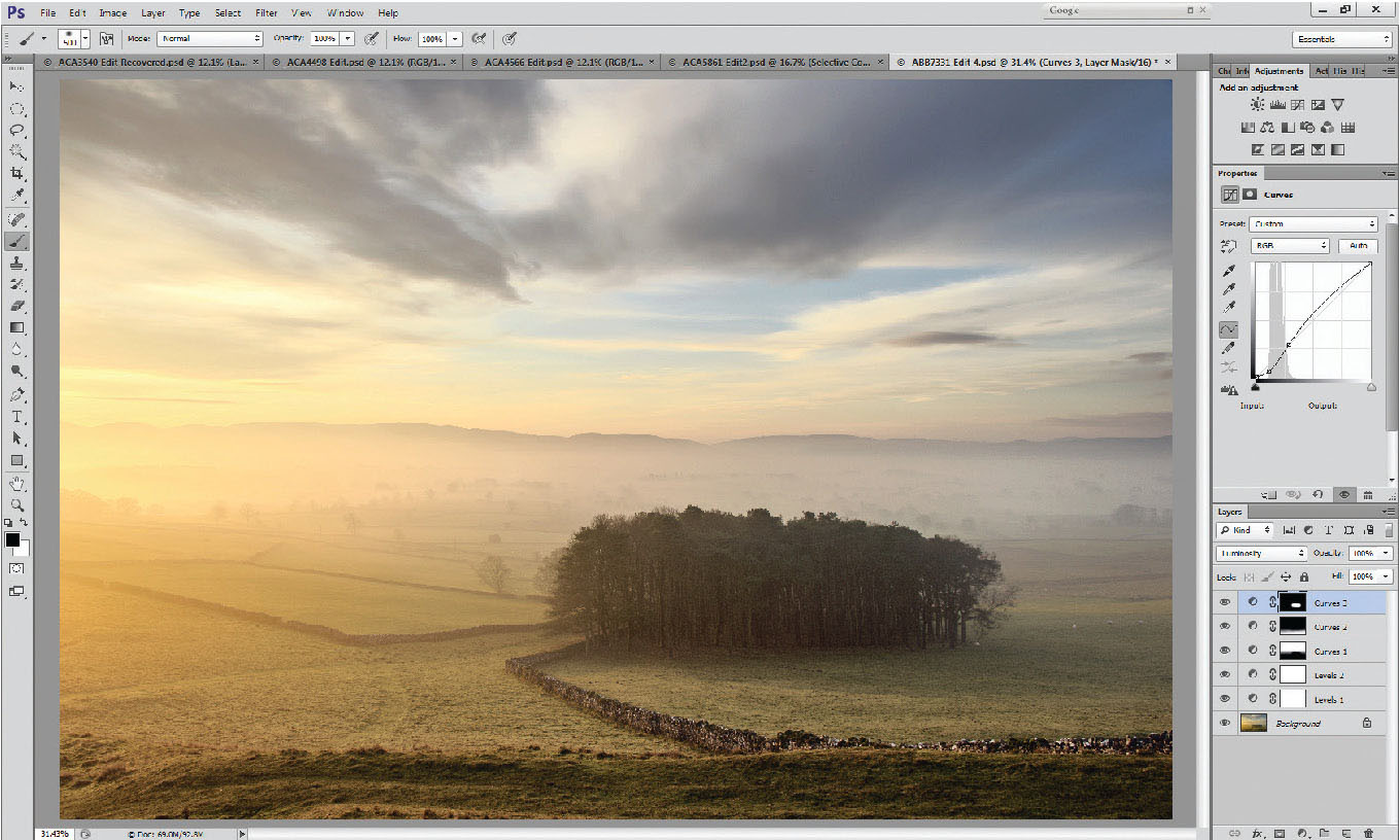
Fig. 4.14
Curves layer added to copse to lighten the tones of the trees and increase the separation of tones therein.
Next, select the ground (excluding the copse), in a similar manner.
And again using curves, add a little localized contrast to this area – how you change the contrast is up to personal interpretation. In this case, by steepening the curve through the histogram, but keeping the darker tones unchanged, the feeling of frost on the ground has been emphasized.
Next, select the trees in a similar manner, using quick mask (Q) and a brush tool (B) – black brush – to select the area with a very soft edge. Without blocking the shadow details too much in the dark areas, give the copse a touch more ‘bite’ by adding (another) curves layer and carefully increasing the steepness of the curve. Remember, with all these adjustments it’s important to make the changes subtly, so they are imperceptible to the viewer.
Equally important at every stage is to stand back and look at the photograph, to see if the balance of the picture remains in harmony, or if it has become imbalanced. In this instance, the left-hand edge is looking a little over-bright, so further work is needed there. A selection of the left side (you can use a gradient tool, or a very large brush, or a combination of the two; maybe by taking a gradient of the left side of the image, then removing part of the selection by using a white brush), possibly taken in two selections – the sky and the land. Add separate curves layers to these and work them individually. The sky selection can take some darkening, just to bring those bright areas of sky down to a similar tonality to the rest of the sky and stop the viewer’s eye from being drawn to the light areas at the corner of the print. Try changing the blending mode to luminosity to avoid increasing the saturation in those areas as well.

Fig. 4.15
Changes to the sky and land (Curves layers 4 and 5) to the left of the picture, layer 4 to increase definition within the clouds by increasing contrast slightly without unduly lightening the tones, layer 5 on the ground to again increase depth and separation, but lightening the tones slightly to emphasize the early-morning feel.
The ground area needs a touch more contrast – focused on the tones of the walls, to make them stand out more from the field; the adjustment can be almost imperceptible, but all these little stages make a huge difference to the final picture.
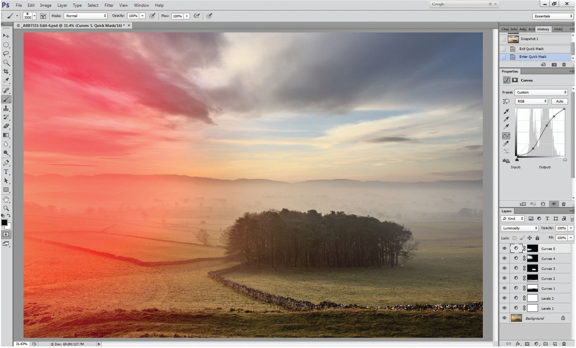
Fig. 4.16
Selection of yellow areas of sky and land with quick mask/brush tool, using a very soft-edged and large brush (3000 pixels wide).
The left-hand side of the photo now balances the rest, but the strong yellow tones still present might not be to everyone’s taste. Using the brush tool in quick mask (Q) make a very soft-edged selection of the predominantly yellow areas. As the larger soft-edged brushes give a softer edge than the smaller brush sizes, try using a brush diameter of about 2,000 pixels. Remember, the brush size can be adjusted using the square brackets, and the brush hardness by using Shift>square brackets.
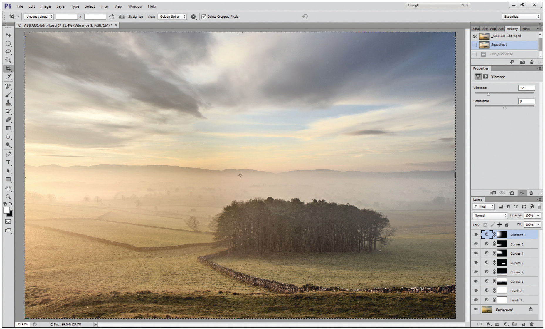
Fig. 4.17
Vibrance reduced to the yellow tones on the left of the picture to portray the frosty cold feel across the image.
Exit quick mask (Q) and based on this selection, add a vibrancy layer. Try reducing the vibrancy until the vivid yellow becomes more in keeping with the frosty, misty feel of the morning. This example took it down to 40 (Figure 4.17). Vibrance is better for this type of adjustment than hue and saturation, as it preserves the saturation of the less dominant tones, just subduing the brighter colours. For those on Elements rather than Photoshop, you don’t have the advantage of the vibrance layer, so might have to use a hue and saturation layer. If this is the case, select from the hue and saturation options; the ‘master’ drop-down menu allows you to select primary (red, green and blue) or secondary (cyan, magenta or yellow) colours. Choose yellow, and reduce the saturation – in this case, −25 seemed about right, but the adjustment is subjective – it’s all a matter of personal taste, the important thing is not to overdo it at any stage and just to move things forward a bit at a time.