12: DAX Topic: VALUES(), HASONEVALUE(), SELECTEDVALUE(), and CONCATENATEX()
In Chapter 9 I introduced the idea that CALCULATE() can use two types of filters: simple filters and advanced filters. Simple filters are in this form:
TableName[ColumnName] = some value
On the other hand, an advanced filter takes a table as a filter input. In other words, you use an existing table (or create a virtual table on-the-fly) that contains the rows you want included in the filter, and CALCULATE() applies that filter to the data model before completing the evaluation of the main expression.
The tables you create using functions can be thought of as being “virtual” because they are not physically stored as part of the data model. They are created on-the-fly inside your DAX formulas and can be used during the evaluation of just the specific formulas containing the virtual table. Importantly, when you create a virtual table using a formula, the new virtual table will have a virtual relationship to the data model, and that virtual relationship will propagate the filter context in exactly the same way that the permanent relationships do. (You’ll learn more about this later in the chapter.) Virtual tables are said to retain lineage with their source tables.
VALUES() is the first function you have come to in this book that returns a (virtual) table. If you type the word VALUES into the formula bar and read the tooltips, you can see that this function returns a table, as shown below.

One important thing to note about VALUES() is that it respects the initial filter context coming from your visuals. So if you combine this fact that VALUES() respects the current filter context with the information provided by IntelliSense in the image above, you will see that VALUES() returns a single-column table that contains the list of all possible values in the current filter context.
It’s time to work through some examples to demonstrate the point.
A Calendar Example
Set up a new matrix as shown below and put Calendar Year on Rows. Then write the following measure in the Calendar table:
= COUNTROWS(
VALUES('Calendar'[MonthName])
)

Note: The following formula does not work here:
Total Months in Calendar wrong
= COUNTROWS('Calendar'[MonthName])
This formula doesn’t work because COUNTROWS() expects a table as the input, but ‘Calendar’[MonthName] is not a table; rather, it is a column that is part of a bigger table (the Calendar table, in this case).
When you wrap 'Calendar'[MonthName] inside the VALUES() function, this single column that is part of the Calendar table is converted into a table in its own right, and it retains a relationship (lineage) to the original Calendar table. This new table returned by VALUES() is still a single column, but now it technically is a table and a column instead of simply being a column of some other table (Calendar, in this case).
So VALUES('Calendar'[MonthName]) returns a single-column table of possible values that respects the initial filter context coming from the matrix. It is not possible to put this new table created by VALUES() into a measure unless you wrap it inside some other formula (e.g., an aggregator). In the example above, you first create the table (the VALUES part of the formula) and then count how many rows are in the table by using the COUNTROWS() function:
Total Months in Calendar
= COUNTROWS(
VALUES('Calendar'[MonthName])
)

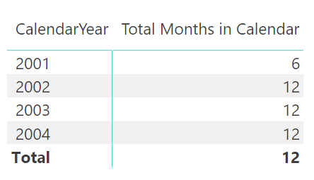
Notice how the year 2001 has only 6 months, and the other years all have 12. This is proof that the VALUES() function respects the initial filter context from the matrix. The initial filter context for the first row in the matrix is 'Calendar'[Year] = 2001. That filter is applied before the formula [Total Months in Calendar] is calculated. VALUES() takes this “prefiltered” table (only dates where the year = 2001 are left unfiltered) and returns a single-column table that contains a distinct list of the possible values.
Returning a Single Value
VALUES() returns a single-column table of unique values from another column in another table, and this new table of values respects the current filter context coming from the visual in the report. There is another very cool feature of VALUES() that is very powerful: In the special case where VALUES() returns just a single row (i.e., one value), you can refer to this value directly in your formulas.
If you take the example created above, remove CalendarYear from Rows, and put MonthName on Rows instead, you should get the following.

Now you can see below that with the exception of the grand total, each row in the matrix has only a single value for [Total Months in Calendar]. So as long as you write the formula in such a way that it operates over only a single row of the table, you can create a measure that returns the name of the month into the matrix’s Values section (i.e., not Rows or Columns).

To write this formula, you need to provide protection for the other possible scenario, where VALUES('Calendar'[MonthName]) has more than one row in the table. This is done using the function HASONEVALUE(), like so:
Month Name (Values)
= IF(HASONEVALUE ( 'Calendar'[MonthName] ),
VALUES( 'Calendar'[MonthName] )
)
Remember that the structure of an IF() statement is as follows:
= IF(Logical Test, Result if True, [Result if False])
The last parameter is optional. If you leave it out, then you are accepting the default value, BLANK().
If you write the above formula without the HASONEVALUE() function, it will throw an error. Even if you remove the grand total from the matrix, it will still throw an error. DAX allows you to use the single value returned in a single row of the single-column table only if you protect the formula with HASONEVALUE().
The New SELECTEDVALUE() Function
In August 2017, Microsoft released a new function in Power BI, called SELECTEDVALUE(). You may recall that earlier I discussed the concept of syntax sugar—an approach Microsoft developers use to make difficult formulas easier to use. Here is the syntax for SELECTEDVALUE():
SELECTEDVALUE(ColumnName, AlternateResult)
SELECTEDVALUE() was created to replace the complex formula in the previous section. Here is the formula from above:
Month Name (Values)
= IF(HASONEVALUE ( 'Calendar'[MonthName] ),
VALUES ( 'Calendar'[MonthName] )
)
The new SELECTEDVALUE() function allows you to rewrite the same formula as follows:
Month Name Alternate
= SELECTEDVALUE ( 'Calendar'[MonthName] )
Under the hood, SELECTEDVALUE() performs the IF HASONEVALUE test, and it returns the single value in the column if there is just one. AlternateResult is BLANK() by default.
Note: This new function is not available in Power Pivot for Excel at the time of this writing, so you need to use the previous pattern when using Excel.
Power BI has a special DAX function called CONCATENATEX() that iterates over a list of values in a table and concatenates them together into a single value. By using this function, you can write a formula that returns the single value when there is just one value but concatenate all the values into a single value when there are multiple values. You could write the earlier VALUES formula like this:
Month Name (Values)
= CONCATENATEX(VALUES ( 'Calendar'[MonthName]),
[MonthName],", ")
With this formula, you get the result shown below.

Here’s How: Changing the MonthName Sort Order
In the example above, you can see that the month names in the matrix are sorting in alphabetical order rather than in the logical month order of a calendar year. By default, all columns in all tables sort in alphanumeric order. It is, however, possible to change the sort order.
Follow these steps to change the sort order in a table:
1. Go to Data view and navigate to the Calendar table.
2. Click in the MonthName column (see #1 below), click the Sort by Column button (#2), and then select the MonthNumberOfYear column to be the sort column (#3).

3. When you return to your matrix, the rows are sorted in logical month order, as shown below.

Note: Even though the columns are now sorting in the correct month name order, the concatenated value in the total row does not sort correctly. There is an optional OrderBy parameter available inside CONCATENATEX(), but it is not well documented and is difficult to use in this scenario. I therefore do not provide a solution to this problem in this book.
It is best practice to always load a numeric column in your lookup table for every alphabetic column that needs to be sorted in a different order. You should therefore always include a numeric column in your Calendar table for days of week as well as months of year.
Note: When you create a numeric sort column in a table, there must be a one-to-one match between the values in the numeric sort order and the values in the column to be sorted.
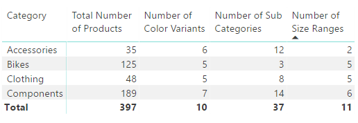
Create a new matrix and put Products[Category] on Rows and the measure [Total Number of Products] on Values. Then write the following measures by first creating a VALUES() table and then wrapping this table inside a COUNTROWS() function, as in the example shown earlier in this chapter. Find the solutions to these practice exercises in "Appendix A: Answers to Practice Exercises" on page 214.
39. [Number of Color Variants]
40. [Number of Sub Categories]
41. [Number of Size Ranges]
Use the column Products[SizeRange] for this one.
You should end up with a matrix that looks like the one below.

Note: Each of these measures is the equivalent of dragging the column name and dropping it into the Values section of the matrix. When you drop a text field into the Values section of a matrix in Power BI, the matrix creates an implicit measure and uses COUNT() as the aggregating method. But recall that I recommended that you avoid doing this. The names created by implicit measures are ugly, and you need the DAX practice, so instead I recommend that you write explicit DAX measures, particularly while you are learning.
Business users (i.e., those who don’t have a professional IT background) often find it somewhat difficult to understand the VALUES() function because you can’t actually “see” the table. So far I have shown you that even though you can’t see the table, you can wrap the table inside a COUNTROWS() function—so at least you can see the number of rows in the table.
Power BI Desktop has a feature called New Table that is not currently available in Power Pivot for Excel. The New Table button is on the Modeling tab (see #1 below).

When you click this button (#2), you see that you can write a formula in the formula bar (#3). When you create a new table using this button, you can write a formula that returns a table (e.g., VALUES()), and the table is added to the data model.
Say that you write a table with the following DAX formula:
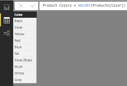
Product Colors = VALUES(Products[Color])
You get the new table shown below in the data model (visible in Data view).

Recall that VALUES() returns all the unique values in the current filter context. A new table doesn’t respond to filters from Report view, so there is no initial filter context for a new table. The table above therefore shows a complete list of all possible values for Product[color] in the entire Products table (no filters applied).
The New Table button is very useful for “materialising” any virtual table so you can “see” the contents of the table. Later in the book, I will show you how you can add your own filter to one of these tables so you can see a subset of a table with a filter applied. For now, it is just good to know that if you ever can’t get your head around a virtual table, you can always materialise it by using this feature so you can take a peek, and then you can delete it when you are done.
Practice Exercises: VALUES(), Cont.
Next, you should use the same matrix from the Practice Exercises 39–41 but remove the measure [Number of Size Ranges] from the matrix. Then write the following measures that each return a single value (the text name) into a cell in the matrix. Each formula has the word (Values) in the name, so it is clear that the formulas are returning the actual name value to the matrix; this is just a “note to self.” In each example, make sure you wrap your VALUES() function in an IF() or HASONEVALUE() function, as in the example earlier in the chapter. Alternatively, you can use the SELECTEDVALUE() function if you prefer.
42. [Product Category (Values)]
43. [Product Subcategory (Values)]
44. [Product Color (Values)]
When you have finished, your matrix should look as shown below. Notice that two of these measures are blank. This is because the VALUES formula has more than one value, and hence the IF HASONEVALUE (or SELECTEDVALUE) part of the formula returns BLANK(); this is the default if you omit the last parameter.

45. Modifying Practice Exercise 43
Try editing the IF() statement for [Product Sub Category (Values)] so that it returns the value More than 1 SubCategory instead of BLANK(). The syntax for IF is IF(Logical Test, Result if True, Result if False).
46. Modifying Practice Exercise 44
Now try editing the IF() statement for [Product Color (Values)] so that it returns More than 1 Colour instead of BLANK(). You should end up with something like the following (which shows answers for Practice Exercises 45 and 46).

Finally, add a couple of slicers to your report from the Products table for color and subcategory.
Note: If you add a slicer on a numeric column, it will look different to mine below. You can change the way a slicer displays from the drop-down arrow menu in the top-right corner of the slicer visual.
When you click on these slicers, the values in the matrix update to reflect the filtering in the slicer(s).
