13: DAX Topic: ALL(), ALLEXCEPT(), and ALLSELECTED()
The DAX functions ALL(), ALLEXCEPT(), and ALLSELECTED() are all very similar in what they do. Let’s start with ALL() and then look at the other two variants.
The ALL() function removes all current filters from the current filter context. For this reason, ALL() can be considered the “remove filters” function. The easiest way to understand this is with an example.
Create a new matrix and put Products[Category] on Rows and put the [Total Number of Products] measure you created earlier on Values. You get the matrix shown below.

Technically what is happening above is that the first row in the matrix is filtering the Products table so that only products that are of type Products[Category]="Accessories" are visible in the underlying table; the other products are all filtered out. They are not really visible, but you can imagine what the underlying table in your data model would look like with a filter applied to Accessories behind the scenes. After the matrix applies a filter to the underlying tables, the measure [Total Number of Products] counts the rows that survive the filter. It does this for every cell in the matrix, one at a time, including the total cell. There is no filter applied to the total cell, so the measure counts all rows in the table (a completely unfiltered copy of the table).
Now create a new measure that uses the ALL() function:
Total All Products = COUNTROWS(ALL(Products))
The ALL() function returns a table. You can’t see the table, but you can wrap COUNTROWS() around it so you can see how many rows are in the table. As you type this formula, if you pause while typing, IntelliSense displays the syntax for ALL(), as shown below.

In this case, IntelliSense is saying you that you can pass either a table or a single column as the first parameter for ALL(). In this example, you are passing the entire table. When you have finished typing this formula, add the measure to your matrix, and you should get the results shown below in your matrix.

You can see from this matrix that the new measure (the one on the right) is ignoring the initial filter context coming from the rows in the matrix. What is happening here is that first of all, the initial filter context is set by the row Products[Category], but the ALL() function always returns an unfiltered copy of the table, and hence it returns the entire Products table instead of the filtered Products table. So COUNTROWS() returns 397 for every row in the matrix—including the total, as before.
Using ALL() as an Advanced Filter Input
The most common use of ALL() is as an advanced filter table input to a CALCULATE() function. Let’s look at an example using ALL() as a table input to CALCULATE().
A good use for ALL() inside CALCULATE() is to remove the filters that are naturally applied to a visual so that you can access the number that is normally in the total line of the visual. Once you can access the equivalent total in a visual (such as a matrix) from any row in the matrix, you can then easily create a measure that finds the percentage of the total, which would be very useful indeed. The concept will make more sense as you work through the following example.
Calculating the Country Percentage of Total Sales
Say that you want to calculate the country percentage of global sales. First of all, set up a matrix with Territories[Country] on Rows and [Total Sales] on Values, as shown below.

It is then possible (as shown below) to select the matrix (see #1 below), click on the drop-down arrow next to the measure [Total Sales] (#2), and then select Show Value As (#3) and Percent of Grand Total (#4).

But if you do this, you are only changing the display format of the result and not actually calculating the percentage as part of your data model. This means you can’t use these percentages inside other measures, and you also can’t reference the percentages from cube formulas (discussed in Chapter 19). Of course, you are also not learning to write DAX!
Writing Your Own DAX Measures
As illustrated in the preceding section, it is much better practice to create a new measure that will return the actual value as a reusable asset in your data model. You can do this in two steps.
Tip: Remember that it is good practice to break the problem you are solving into pieces and solve one piece of the puzzle at a time.
Step 1: Create a Grand Total Measure
Right-click the Sales table and create the following new measure:
Total Global Sales
= CALCULATE([Total Sales] , All(Territories) )
Don’t forget to apply suitable formatting immediately, before moving on.
As you know, the first parameter of CALCULATE() is an expression, and the subsequent parameters are filters that modify the filter context. In this case, you are passing a table as the filter context. This table is ALL(Territories), which is actually an unfiltered copy of the entire Territories table.
After you add the new measure to the matrix, your matrix looks as shown below. Do you see that the new measure is ignoring the initial filter context coming from the matrix? CALCULATE() is the only function that can modify the filter context. In this case, CALCULATE() is replacing the initial filter context on Territories[Country] with a new filter context (an unfiltered copy of the Territories table).

Step 2: Create the Percentage of Total
After you have created the measure [Total Global Sales], it is easy to create a new measure to calculate the country percentage of global sales, as follows:
% of Global Sales
= DIVIDE([Total Sales] , [Total Global Sales])
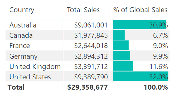
Make sure you format this measure so that Format is set to Percentage and Decimal Places is set to 1. You end up with the matrix shown below.

The final step is to remove the [Total Global Sales] measure from the matrix.
Note: You don’t actually need the interim measures you write to be placed in the matrix in order for the [% of Global Sales] measure to work. But you should notice how much easier it is to visualise what is happening when you write these measures in the context of a matrix. When you do it this way, you can easily see how the [Total Global Sales] value is the same, regardless of the country in the matrix, and hence you can immediately see that you just need to divide the country sales by this total global sales amount, and it is going to work.
The final matrix is shown below, with some conditional formatting applied to make it easier to read.
Using the Quick Measures Option
You may already know—or may have noticed in one of the earlier images—that there is a New Quick Measure option available in Power BI. If you click the drop-down button next to Total Sales (see #1 below), you see the New Quick Measure option (#2).
Note: At this writing, Quick Measures is still in preview. If you can’t see the New Quick Measure option in the menu (as shown below), you can turn this preview feature on via the following menu: File\Options and Settings\Options\Preview Features\Quick Measures

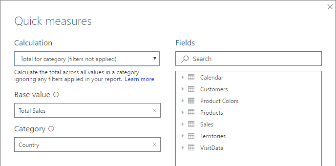
If you select the New Quick Measure option, Power BI will help you write a measure, and you don’t have to have any knowledge DAX at all. Using New Quick Measure is much better than creating implicit measures, as discussed earlier in this chapter. Some reasons are that you can rename the measure, edit the measure, and reuse the measure inside other measures. The image below shows Total for Category (Filters Not Applied) selected for the calculation in a new quick measure. All you have to do is drag a column or measure from the fields list on the right into the relevant placeholders on the left. In the example below, I have added [Total Sales] to Base Value and Territories[Country] to Category.
Note: Did you notice that I didn’t need to tell you that [Total Sales] is a measure and Territories[Country] is a column? This is best practice at work. You should always omit the table name from the measure and always include the table name in front of a column; if you do, others in the DAX authoring community will understand what you mean.
The measure that Power BI creates is shown below.

Note that this is a real measure—almost identical to the one that was hand-written above. However, at this writing, the New Quick Measure feature is not using best practice. Can you spot what is wrong with the measure above? The first parameter in CALCULATE() is a measure, but the measure is referencing the table name before the measure name. You should never do this—never ever! Always add the table name before a column name; do not add the table name before a measure name. The good news, however, is that because this is a real measure, you can simply edit what the New Quick Measure feature created and correct the syntax yourself. (I expect that this “poor practice” will be fixed at some point in the future. I have already reported it to Microsoft.)
Note: Using the New Quick Measure option is a great help for writing more complex DAX functions quickly and without a lot of knowledge about how it all works. However, I do not spend any more time talking about the feature in this book because this is a book about writing your own DAX formulas. If you want to use New Quick Measure, then do so by all means. I don’t recommend that you use New Quick Measure in place of learning how the DAX language works; rather, I recommend that you use New Quick Measure as a tool to help you learn the DAX language.
Passing a Table or a Column to ALL()
Before we finish with ALL(), it is worth pointing out that this next measure would return exactly the same result as [Total Global Sales] in the matrix example in the section “Step 1: Create a Grand Total Measure,” above:
Total All Country Sales
= CALCULATE([Total Sales],
ALL(Territories[Country])
)
Notice that this measure passes a single column instead of the entire table to the ALL() function. So in this specific matrix (shown below), the values for [Total Global Sales] and [Total All Country Sales] are identical.

However, the measure [Total All Country Sales] would not work (i.e., it would not remove the filter) if there were some other column on Rows in the matrix (i.e., something other than Country). To test this, remove Territories[Country] from Rows in the matrix and replace it with Territories[Region]. You get the result shown below.

Notice the difference between passing the entire table name to the ALL() function and passing a single column. [Total Global Sales] removes the filter from the entire Territories table, but [Total All Country Sales] removes filters only from the Territories[Country] column of the table. In the image above, there is no filter on the Territories[Country] column of the table, and hence ALL() has no effect on the visual.
Remove [Total All Country Sales] from the matrix before proceeding.
The New Table Option Revisited
Now is a good time to revisit the New Table feature introduced earlier in the book. Remember that you can use the New Table button (see #1 below) to “materialise” a table into the data model. Normally you can’t “see” a table function in a DAX formula, and that makes it hard to understand what the table function is doing. But if you take the table function and add a new table, as shown below, you can actually see the table that is generated.
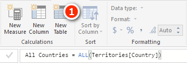
After creating the table above, switch to Data view and click on the new table. You can see that this table consists of a list of six countries plus NA.

This table is just a test table. It isn’t connected to the data model at all, but it can be if you want to connect it. I just like to materialise tables like this as part of the learning experience because it is helpful to be able to visualise table functions. You should delete such test tables when you are done so you don’t get confused.
The ALLEXCEPT() Function
ALLEXCEPT() allows you to remove filters from all columns in a table except the ones that you explicitly specify. Consider the following example:
Total Sales to Region or Country
= CALCULATE([Total Sales],
All(Territories[Region],Territories[Country])
)
ALLEXCEPT() solves the problem implied above, where you need to specify many columns individually in the case that you want most but not all columns in your formula. The above formula works when you have Territories[Country] on Rows and also when you have Territories[Region] on Rows, but it does not work with Territories[Group] on Rows. If you have a lot of columns in your table, you have to write a lot of DAX code to make such a formula work for all but a few of the columns. This is where ALLEXCEPT() comes into play. The above formula can be rewritten as follows:
Total Sales to Region or Country 2
= CALCULATE([Total Sales],
ALLEXCEPT(Territories, Territories[Group]))
Note: You must first specify the table that is to be included and then specify the exception columns.
The ALLSELECTED() function is useful when you want to calculate percentages, as shown above, and you have a filter applied (say, via a slicer) but you want the total in your matrix to add up to 100%.
Say that you’re working with the same matrix used earlier in this chapter but now with a slicer that filters on Territories[Group]. Notice below that [% of Global Sales] adds up to 38.7%; this is correct because the other countries that make up the remaining 61.3% have been filtered out by the Group slicer.

But say that you want to see the percentage of each region out of all the values in the matrix (in this example, just the regions in the group North America). This is where ALLSELECTED() comes in. ALLSELECTED() removes the filters from the matrix but respect the filters in the slicer.
Add the following measure to the matrix above:
Total Selected Territories
= CALCULATE([Total Sales], ALLSELECTED(Territories))
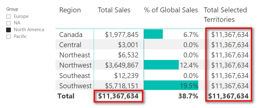
Notice how the interim measure [Total Selected Territories] returns the same value as the total of the items in the matrix. Using the same steps as before, you can now write a new measure [% of Selected Territories] and then remove the interim measure [Total Selected Territories] from the matrix.
Now write the following measure:
= DIVIDE([Total Sales] , [Total Selected Territories])
Remember to format this new measure using percentage and one decimal place.

Remember that it is good practice to split a problem into pieces and solve one piece of the problem at a time. My advice is to get used to creating interim measures first and then writing the final measure that you actually need. Doing this helps you visualise each step of the process and makes it easier to get each part of the end-state formula correct before you proceed to the next step.
It is, of course, possible to write one single measure that does all the steps you just went through. This is what it would look like:
% of Selected Territories ONE STEP
= DIVIDE([Total Sales] ,
CALCULATE([Total Sales],
ALLSELECTED(Territories)
)
)
But this all-in-one formula is much harder to write, read, and debug—particularly when you are learning to write DAX. It’s not wrong; it’s just harder, and life is too short to do things that are harder than they need to be.
Practice Exercises: ALL(), ALLEXCEPT(), and ALLSELECTED()
It’s time for some practice. Create a new matrix and put Customers[Occupation] on Rows and the measure [Total Sales] on Values. You get the matrix shown below.

Then, using the principles covered in this chapter, create the following measures by first creating the interim measure you need and then creating the final measure. Find the solutions to these practice exercises in "Appendix A: Answers to Practice Exercises" on page 214.
47. [Total Sales to All Customers]
48. [% of All Customer Sales]
Now add a slicer for Customers[Gender] to the report you have just created and filter by Gender = M, as shown below.
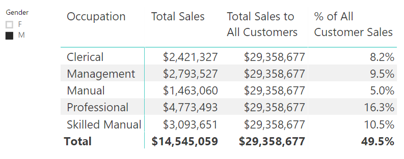
Note how [% of All Customer Sales] doesn’t add to 100%. This is correct because the other 50.5% of customers are filtered out with the slicer.
Set up another matrix with Customers[NumberCarsOwned] on Rows, Customers[Occupation] on Slicer, and [Total Sales] on Values. Your job is to create the other measure in this matrix: [% of Sales to Selected Customers]. When you are done, your matrix should look like the one below, with the last column showing the percentage of sales to customers based on the number of cars they own.
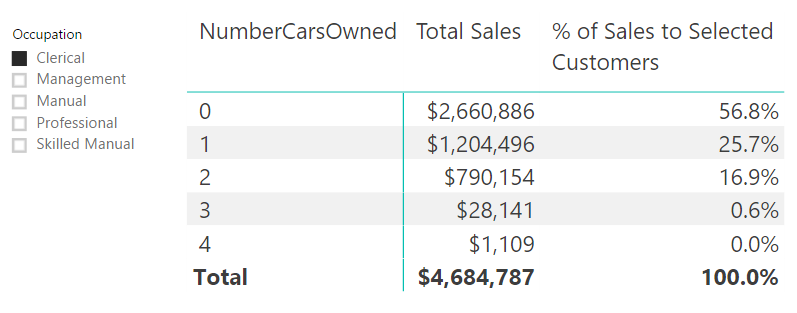
Remember that in this case, you want to create an interim measure first, so you actually need to create the following two measures and then remove the first one from the matrix.
49. [Total Sales to Selected Customers]
50. [% of Sales to Selected Customers]
Create the following two measures. The first one is an interim formula and can be removed from the matrix once you have finished the second formula. Find the solutions to these practice exercises in "Appendix A: Answers to Practice Exercises" on page 214
51. [Total Sales for All Days Selected Dates]
52. [% Sales for All Days Selected Dates]
I don’t use ALLEXCEPT() much, and you may not either, but it is still good to work through an example of how it can be used. This section will give you some practice while also demonstrating one possible use case.
Say that you want to compare the percentage of sales across all occupations and see how it changes depending on the other customer filters. Follow these steps:
1. Set up a new matrix and place Customers[Occupation] on Rows.
2. Add slicers for Gender and NumberCarsOwned.
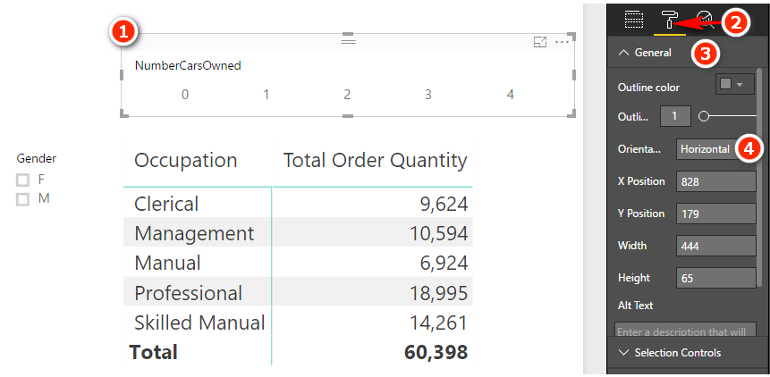
3. Put [Total Order Quantity] on Values. You should have the setup shown below. Note that the total order quantity will change as you click on the slicers.
Here I have set the NumberCarsOwned slicer to be horizontal by selecting the slicer (see #1 below), going to the Format pane (#2), selecting General (#3), and then setting Orientation to Horizontal (#4).
A number of steps are required to get to the end state (which is shown below). The following practice exercises show the measures you need to create, in the proper order, to get to the end state. As you create each measure, check that the results you see in your matrix make sense. Once again, this is the reason to write DAX in the context of a matrix: It makes it easier to get your head around what you are doing.
The following matrix shows all the measures you need to write so you have an overview of what you’ll accomplish with the following measures. Note that there are some slicers applied to the report already.

The image below shows the end state you are working toward, with just the final measures included.

As you can imagine, with this matrix, it is possible to select different combinations of gender and number of cars and then compare the variation between the baseline order quantity and the order quantities for the selected filter.
Practice Exercises: ALL(), ALLEXCEPT(), and ALLSELECTED(), Cont.
Write the following DAX formulas one at a time and check to make sure each looks correct before moving to the next one. Find the solutions to these practice exercises in "Appendix A: Answers to Practice Exercises" on page 214.
53. [Total Orders All Customers]
To check this measure, click on the slicers and note that [Total Order Quantity] should change, but [Total Orders All Customers] should not change based on the slicers.
54. [Baseline Orders for All Customers with This Occupation]
This measure should also not change when you make changes to the slicers. However, note that you should get a different value for each occupation—unlike with [Total Orders All Customers] above. This will be the baseline for comparison.
55. [Baseline % This Occupation of All Customer Orders]
This measure converts the baseline measure above into a percentage of the baseline for all orders. The description of this measure should help you work out how to write the DAX. Test the slicers again and make sure this new baseline percentage doesn’t change with the slicers.
56. [Total Orders Selected Customers]
This measure should adjust depending on the selections you have in the slicers. Hint: Use ALLSELECTED().
57. [Occupation % of Selected Customers]
You can use the interim measures above to create this measure. Click the slicers a few times and see which values change. This new measure should change based on the values you select in the slicers.
58. [Percentage Point Variation to Baseline]
This measure is the percentage of selected customers (Practice Exercise 57) minus the baseline (Practice Exercise 55).
Now you should have an interactive report that allows you to drill into customer attributes (gender and number of cars owned) to see the impact on the mix of business vs. the baseline of all customers.
It is worth pointing out here that sometimes it may be useful to change the descriptions of the final measures as they appear in a matrix. So while [Baseline % This Occupation of All Customer Orders] is a good name for your measure because you know what it means, when you use this measure in a specific matrix, it may be a good idea to rename it. You can do this by selecting the matrix, going to the Values section on the right-hand side of the screen, and double-clicking the measure name you want to change. The name changes just for this single visual (the matrix in this case).
After giving your measures new names, you might end up with something like the matrix shown below.

Note: If you change the description in the matrix, the easiest way to change it back is to remove the measure from the visual and then add it back again.