16: DAX Topic: RELATED() and RELATEDTABLE()
The functions RELATED() and RELATEDTABLE() are typically used in calculated columns to reference relevant records in other tables, although they can be used in measures, too. They are a bit like VLOOKUP() for tables that have a relationship. As mentioned briefly in Chapter 10, a row context does not follow a relationship. So even though there may be a relationship between two tables, a row context cannot use this relationship—unless you use one of these two functions that can. Basically, RELATED() and RELATEDTABLE() allow a row context to leverage an existing relationship so it can access columns in related tables.
When to Use RELATED() vs. RELATEDTABLE()
To understand when to use the RELATED() and RELATEDTABLE() functions, you need to understand what each one returns. As you know, you can use IntelliSense in the formula bar to find out what each of these functions returns.
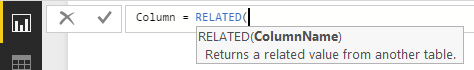
You can see below that RELATED() returns a single value from another table.
As shown below, RELATEDTABLE() returns a table.

Remember from Chapter 2 that relationships between tables in Power BI are normally of the type one-to-many. Also remember from Chapter 2 that best practice (especially for people coming from an Excel background) is to lay out tables in Relationships view with the lookup tables at the top (the “one” side of the relationship) and the data tables at the bottom (the “many” side of the relationship), as shown below.
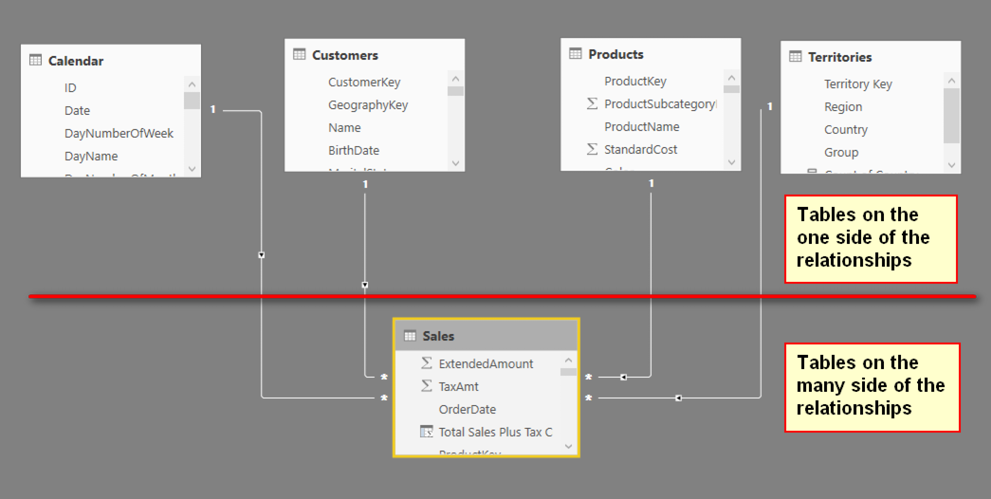
The two RELATED functions allow you to refer to columns in another connected table. So when you think about it, if you want to add a custom column in a table on the “one” side of the relationship—i.e., add a new column in a lookup table (a table above the line in the image above)—then it is highly likely that there will be multiple rows on the “many” side of the relationship. So when writing a formula in a calculated column on a lookup table, you must use the RELATEDTABLE() function because it will fetch a table of values, including all the matching values in the data table. Conversely, if you are writing a calculated column in a table on the “many” side of the relationship (i.e., a data table), then there will be only one matching row in the lookup table, and hence you use RELATED() to return that single value.
The RELATED() Function
This section provides an example of bringing a value from a column in a lookup table into a table on the “many” side of the relationship. For the sake of this example, assume that your business has a new management layer, and you want to add a new level of reporting to cover this new management layer. In effect, you need to enhance the Territories table to add a new geographic region. To achieve this, you could do the following:
1. Create a new table that contains the logic of the new management layer.
2. Import the new table into the data model.
3. Join the new table to the existing Territories table (in this example).
4. Create a new calculated column in the Territories table (on the “many” side of the relationship) and bring in the new management layer from the new table into the Territories table as a new column.
This will all make more sense as you work through the following example, which also shows how you can manually add new tables of data in Power BI.
Here’s How: Manually Adding Data to Power BI
This example shows how to add data directly into Power BI without having to use another tool like Excel:
1. On the Home tab in Power BI Desktop, click Enter Data.
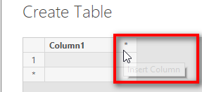
2. As shown below, click the * to add a new column.
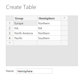
3. Change the column names (double-click them and type a new name) and then enter the data as shown below. Rename the table Hemisphere and then click Load.
4. Switch to Relationships view and rearrange the new tables so that the new table is sitting above the current Territories table, as shown below. This new lookup table is a lookup table to another lookup table and will be on the “one” side of the new relationship. Power BI should automatically join the tables.

Note: The Territories table now has two roles. It is now acting as a lookup table to the Sales table and as a data table to the new Hemisphere table.
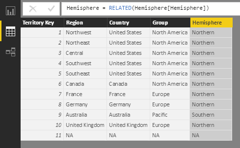
5. Bring the data that resides in the Hemisphere[Hemisphere] column into a new calculated column inside the Territories table. Switch to Data view, right-click on the Territories table, select New Column, and then type in the formula shown below. After you press Enter, you see all the values appear in the new calculated column. It is a lot like VLOOKUP()!
6. Finally, to hide the Hemisphere table from the client tools, in Data view, right-click the table (see #1 below) and select Hide in Report View (#2).
It is good practice to bring data from an add-on table like this Hemisphere table into the main Territories table as an additional column rather than use the data in an additional lookup table. It is possible to leave the Territories table untouched and use the columns from the Hemisphere table in your matrix. But the problem is that this can be confusing to users. It doesn’t make business sense to have all the geographic information in the Territories table except for the hemisphere information, which is in the Hemisphere table. So for consistency and simplicity for the end user, it is better to bring all the “like data” into the same table.
Note: Better practice is to do this when you load the data using Power Query, but you can also do it as shown here. And best practice is to change the Territories table back at the source to include the new Hemisphere column in the Territories table, but that is not always possible in a timely manner.

As discussed earlier, RELATEDTABLE() is used to reference a table on the “many” side of the relationship. A simple example is to add a new calculated column to count how many sales there have been for each product. Once again, I generally don’t recommend that you do this (because you can do it in a measure), but there may be valid reasons to do it in some cases.
Go ahead now and add the following calculated column in the Products table:
= COUNTROWS(RELATEDTABLE(Sales))
As you know, RELATEDTABLE() returns a table, and COUNTROWS() counts the rows in that table. This calculated column in the Products table therefore takes the row context in the calculated column and leverages the relationship with the Sales table to count the rows in the Sales table for just the single product. As a result, you end up with a new column that indicates the number of items sold (over all time) for each product in the Products table. (The quantity for each line in the Sales table is always 1 in this sample data.)
Note: You do not need to use CALCULATE() with RELATEDTABLE() to force context transition and convert the row context to a filter context. RELATEDTABLE() will work on its own.
One valid use case for using RELATEDTABLE() would be if you want to create a slicer to filter on slow-, moderate-, and fast-selling products. If you want to use a slicer, you must write your DAX as a calculated column. (You can’t place measures in slicers.) You could first create a calculated column and then use the banding technique discussed in the next chapter to group products into slow-, moderate-, and fast-moving products. (Park this thought for now and come back after you have read Chapter 17 if you want to try out this technique.)