19: Concept: Using Analyze in Excel and Cube Formulas
So far in this book, you have consumed and visualised the information from data models in reports inside Power BI. But after you have invested so much time and effort building your Power BI data models, you may want to get to the data by using good old traditional Excel. Fortunately, there is an easy way to do this from PowerBI.com, as long as you have a Power BI Pro licence: You can use Analyze in Excel. Before you can use Analyze in Excel, however, you must first publish your Power BI Desktop file to PowerBI.com.
Note: If for some reason you are not able to publish to PowerBI.com, you can still complete the cube formulas exercises later in this chapter. Simply go to my website,
http://xbi.com.au/localhost, and follow the instructions on how to connect Excel to a local instance of Power BI Desktop running on your PC.
Here’s How: Publishing a Report to PowerBI.com
Follow these steps to publish a report to PowerBI.com:
1. Save the Power BI workbook.
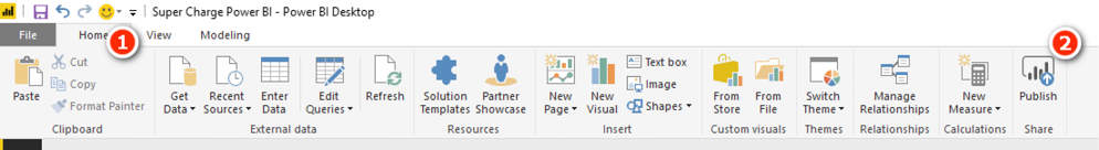
2. On the Home tab (see #1 below), click the Publish button (#2).
3. If this is the first time you are using PowerBI.com, you will be prompted to create an account. Simply follow the instructions to create yourself a new account. If you already have an account, just sign in with your credentials. You get a success message when the file has been loaded to PowerBI.com. If you are creating an account for the first time, you need to activate the 60-day trial in order to use Analyze in Excel.
Note: Your access to PowerBI.com may be controlled by your IT department. If you cannot create an account as described above, you may need to contact your IT department for support. Also, as at this writing, it is not possible to sign up to PowerBI.com using a generic email address such as @gmail.com or @hotmail.com
4. In a browser, navigate to http://powerbi.com and click the sign-in link in the top-right corner of the website, using the same credentials you specified in step 3.
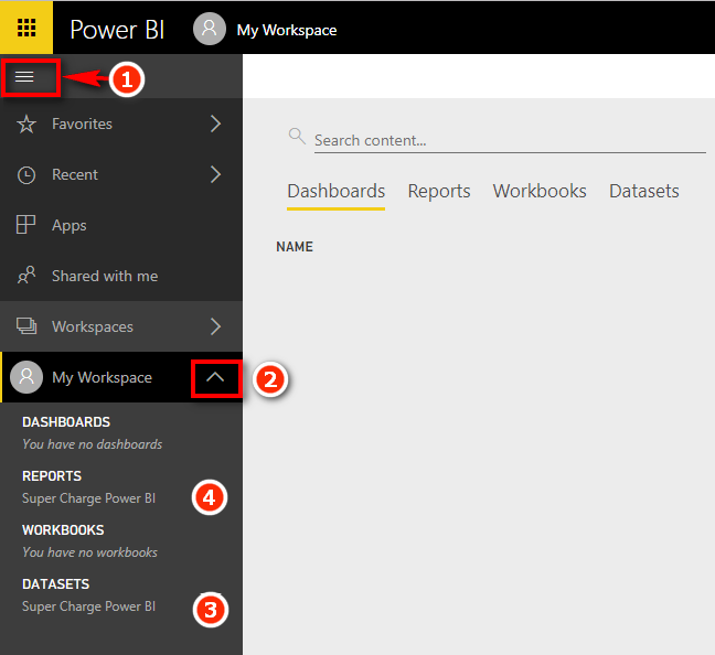
5. Once you are logged in, expand the menu on the left-hand side (see #1 here) and open the workspace where you uploaded your workbook, such as My Workspace (#2).
6. Find your data model under Datasets (see #3 here) and all your reports in the Reports section (#4).
Here’s How: Installing Updates
Before you can use Analyze in Excel the first time, you need to install the Analyze in Excel updates. Follow these steps:
1. Click on the download arrow in the top-right corner of the browser (see #1 below) and select Analyze in Excel Updates (#2).
2. After the update is downloaded, run the downloaded file on your PC. You need administration rights on your computer to be able to complete the installation.
 !
!
Here’s How: Using Analyze in Excel
Using Analyze in Excel could not be easier. Simply follow these instructions:
1. Navigate to either Reports (see #1 below) or Datasets (#2) on the left-hand side and right-click the ellipsis to open the menu and then select Analyze in Excel (#3). An ODC file is then downloaded to your PC.
Note: An ODC file is a small text file that contains a set of instructions to tell Excel how to connect directly to Power BI. You can open an ODC file with a text editor and see what it contains if you are interested.

2. Find the ODC file that was downloaded (probably to your downloads folder, depending on your browser) and click to open it. The figure below shows what this might look like using Google Chrome (bottom left hand corner of the Chrome screen).

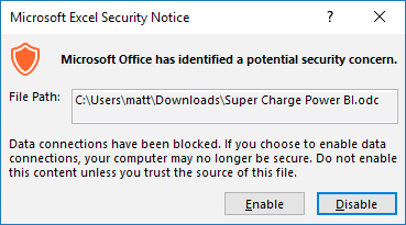
3. If you’re prompted with a security warning when Excel launches, click Enable.
If everything has gone well, you should now have a new pivot table in a new Excel workbook that looks like the one below. You will have to log in again to your account if prompted.

The really cool thing about this Excel workbook/pivot table is that it has a direct connection to PowerBI.com. The data model remains at PowerBI.com, and only the data needed to display the pivot table is stored in the Excel workbook. The data model could be as big as 10 GB on PowerBI.com, but the Excel workbook could be as small as 20 KB. We call these “thin workbooks.”
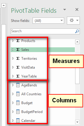
The PivotTable Fields list on the right-hand side of Excel looks slightly different to this list for a regular pivot table. There are measure tables and also column tables, differentiated by the two different icons shown below.
You should be able to build a pivot table similar to one of the matrixes that you have already built in Power BI Desktop. (See the example below.)

The final concept topic in this book is one of my favourites: cube formulas. Cube formulas have been around for many years. But before Power BI was launched, the main way you could use cube formulas was to connect to a SQL Server Analysis Services (SSAS) multidimensional cube. Some large companies have SSAS set up. Some of those companies may connect directly to SSAS from Excel, and some of the ones that do may have discovered cube formulas. But given how rare this scenario is, most people have not come across cube formulas prior to discovering Power BI.
Pivot tables in Excel are great, and I use them all the time, but they do have some limitations. The biggest limitation is that a pivot table locks you into a particular format. But what if you want to put a single value in a single cell in a workbook? In that case, you could create a pivot table and then point the cell in question to the pivot table, but that involves a lot of overhead. In addition, if the pivot table changes shape at any time (e.g., on refresh), then chances are the cell positions will change, and your formula may point to the wrong cell. The best-case scenario is that you realise there is a problem. The worst-case scenario is that your formula points to another similar cell in the pivot table, and you don’t even notice!
“What about GETPIVOTDATA()?” I hear some of you say. Well, yes, you can use GETPIVOTDATA(), but you still have the overhead of the pivot table, and the bottom line is that cube formulas are much better. The easiest way to get started with cube formulas is to convert an existing pivot table to cube formulas. The following pages walk you through how to do that.
Here’s How: Converting a Pivot Table to Cube Formulas
Follow these steps to convert a pivot table to cube formulas:
1. Create a new blank sheet in your Excel workbook and insert a pivot table like the one shown below, which is the same one created in Chapter 18.
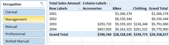
2. Put ‘Calendar’[CalendarYear] on Rows, Products[Category] on Columns, and [Total Sales] on Values. Also add a slicer for Customers[Occupation]. Click on the slicer and make sure it works before proceeding.
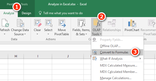
3. To convert the pivot table to cube formulas, click inside the pivot table and then select the Analyze tab (see #1 below), click OLAP Tools (#2), and select Convert to Formulas (#3).
Bam! Your pivot table is converted to a stack of standalone formulas that you can move around as you want on the spreadsheet.

What’s more, the slicer still works! Go ahead and drag the formulas around to new locations in your spreadsheet and then click on the slicer to verify that it works.
Writing Your Own Cube Formulas
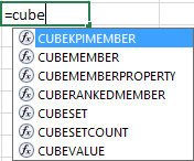
There are seven cube formulas in total in the family, and they all start with the word CUBE. You can see the list by typing =CUBE into a cell in your workbook, as shown below.
This book covers the two most-used formulas, CUBEVALUE() and CUBEMEMBER(). Once you have mastered these two formulas, you can do some research to learn about the other five.
CUBEVALUE() vs. CUBEMEMBER()
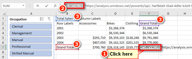
Go back to the pivot table that you just converted and double-click inside the grand total cell (see #1 below) so that Excel is in Edit mode. Notice in the formula bar (#2) that this grand total cell is a CUBEVALUE() formula, and it points to a number of other cells (#3). The formulas inside each of these other cells (labelled #3) are CUBEMEMBER() formulas.
CUBEVALUE() is used to extract the value of a measure from the data model, and CUBEMEMBER() is used to extract a value from a column/lookup table. When they are used together, CUBEMEMBER() filters the data model before calculating the CUBEVALUE() expression.
Now that you know about cube formulas, you can build a pivot table that contains the cube formulas you want in your spreadsheet and then simply select Analyze, OLAP Tools, Convert to Formulas. Once you have done this, you can copy and paste the resulting formulas wherever you want. But it actually isn’t very hard to write cube formulas from scratch, so let’s do that together now.
Here’s How: Writing CUBEVALUE() from Scratch
The important keyboard keys when writing cube formulas are the double quote, the square brackets, and the full stop (period in the USA). This information will make sense as you work through these steps. Be sure to follow these steps exactly:
1. Click in an empty cell in your workbook and type =CUBEVALUE(. Notice the tooltip that pops up, asking for a connection and one or more member expressions. The member expressions can be either measures or table columns from your data model.

2. Type " (a double quote). You are presented with a list of connections available to the workbook. Given that this is a thin workbook created using Analyze in Excel, you should have a connection string that looks something like the one shown below. Note that the long number (GUID) is unique to your instance of Power BI. Anyone who can access your Power BI data set (e.g., someone else in your organisation) will also be able to interact with this thin workbook when it is done.

Note: If you are writing a cube formula using my localhost workbook http://xbi.com.au/localhost, then you will get a different connection string experience than shown above.
3. Press the Tab key to select the connection and then type " again.
4. Type , (a comma).
5. Type " (a double quote) again to start the next parameter. This time notice that the tooltip shows you a list of all the tables in the data model (see below). There is also one additional item in the list, [Measures]. All of your DAX formulas are stored in [Measures].
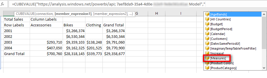
6. Type [ and then M and press Tab to select [Measures].
7. Type . (a full stop/period), and you see a list of all the measures that exist in the data model. From here you can either keep typing [ followed by the name of the measure or use the up and down arrow keys on the keyboard to navigate to the measure you want to select.

8. Type [ and then type Total S. This brings the [Total Sales] measure to the top.
9. Press Tab, type "), and press Enter.
If you follow these instructions exactly, you end up with a value in a cell, as shown below. This is your first handwritten cube formula:
= CUBEVALUE(<your connection string>,"[Measures].[Total Sales]")
Note: In the formula above, I have used <your connection string> in place of the actual connection string because what you have on your screen will be different.
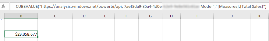
You probably noticed that the value you end up with after writing this cube formula is the grand total for all the data in the data model. It should therefore be clear that the data model is completely unfiltered. It is possible to filter this formula just as in a pivot table by adding some CUBEMEMBER() functions into the formula (sort of like adding a column to Rows in a pivot table).
Note: Before moving on, you should rewrite the formula above a couple of times for practice. Remember that the most important keys on your keyboard in this process are double quotes, square brackets, and the full stop/period, along with Tab to select the highlighted selection. Practice the rhythm of writing these formulas using these keys on the keyboard.
Here’s How: Applying Filters to Cube Formulas
To filter an existing formula, follow these steps:
1. Select one of the formulas you have already written and start to edit it.
2. Delete the last ) and then type , (a comma). The tooltip asks for member_expression2.
3. Type "[.
4. Use the down arrow key to select [Calendar] and then press Tab.
5. Type . (full stop/period) and use the down arrow key to select [CalendarYear]. Then press Tab.
6. Type . (full stop/period) and notice that the tooltip offers only a single choice, [All]. Select [All] and then press Tab.
7. Type . (full stop/period) again and notice that you now have a list of the possible years to select from. Select [2003].
8. Finish the formula by typing ") and pressing Enter.
This is the final formula:
= CUBEVALUE(<your connection string>,"[Measures].[Total Sales]", "[Calendar].[CalendarYear].[All].[2003]")
Go back into this formula again and delete the closing bracket ), add another , (a comma), and then follow the same process as above to add another cubemember, this time for Products[Category] = "Clothing". This is the formula you need:
= CUBEVALUE(<your connection string>,
"[Measures].[Total Sales]",
"[Calendar].[CalendarYear].[All].[2003]",
"[Products].[Category].[All].[Clothing]"
)
You can add any measure from your data model into your spreadsheet by writing a cube formula like this. You can further filter the measure in your cube formula by adding additional CUBEMEMBER() expressions inside the cube formula you are writing.
Here’s How: Adding a Slicer Without a Pivot Table
Connecting your formulas to slicers is easy. You should have a slicer for Customers[Occupation] on the sheet. If you don’t have this slicer, then go ahead and add it now. Here are the steps to add a slicer when there is no pivot table:
1. Select Insert, Slicer.
Note: In this case, you can’t right-click on a column in the PivotTable Fields list because there is no pivot table.
2. In the Existing Connections dialog that appears, select the Connections tab (see #1 below), select Connections in This Workbook (#2), and then click Open.

3. Find the Products[color] slicer in the list, select the correct checkbox, and click OK. You now have a slicer on your sheet, but it is not connected to your formula.
Here’s How: Connecting a Slicer to a Cube Formula
Follow these steps to connect a slicer to a cube formula:
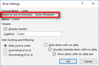
1. Check the unique name for the slicer you want to connect by right-clicking on the slicer and selecting Slicer Settings.
2. In the Slicer Settings dialog that appears, note and memorise the value that appears in the second line in the dialog box, Name to Use in Formulas. You will need the name of the slicer in the next step. In the example shown here, it is called Slicer_Products. In your case, it may be called something different. Once you’ve noted the slicer name, click Cancel.
3. Write a new version of the Total Sales cube formula and this time add the slicer to this formula. Simply add a comma after [Total Sales], followed by the slicer name from step 2, and then type ). Your formula should now look something like this (though your slicer may have a slightly different name):
= CUBEVALUE(<Your Connection String>,
"[Measures].[Total Sales]",
Slicer_Products
)

Note: You do not use double quotes around slicer names. This is an unfortunate inconsistency, but it is just how it works.
4. Now test it out: Click on your slicer and watch your cube formula update.
Take a deep breath and be amazed. How cool are cube formulas?!
In addition to referencing a column name inside a CUBEVALUE() formula, it is possible to write a CUBEMEMBER() formula directly in a cell in a workbook. Here is an example of a CUBEMEMBER() formula:
= CUBEMEMBER(<Your Connection String>,
"[Customers].[Occupation].[All].[Manual]"
)
You can see a lot more of these formulas if you go back to the original pivot table that you converted and click in the column and row headings. If you write a CUBEMEMBER() formula as a standalone formula in a cell, you can reference that cell from within your CUBEVALUE() formula by using cell references. Once again, you can see this by examining the formula in your converted pivot table.