20: Transferring Your Skills to Excel
Power BI is a relatively new product from Microsoft. It first became generally available in July 2015, and the pace of change over the few years since its release has been phenomenal. The fact that you have purchased this book and have now arrived at this point probably means that you already know this. But the truth is that both Power Pivot and Power Query are technologies that were first built (and continue to evolve) for Microsoft Excel. Microsoft didn’t (and still doesn’t) do a really great job at marketing the existence of these products as part of Excel, and as a result, many (most?) people who could benefit from the technologies inside Excel don’t know they exist. The good news, however, is that the skills you have learnt in this book are completely transferable to Power Pivot for Microsoft Excel. This chapter is here to help you transfer those skills with a minimum of pain.
Differences Between Power BI and Power Pivot for Excel
There are a couple of differences between Power BI and the various versions of Power Pivot for Excel that you should be aware of as explained below.
Note: I use the following conventions below:
- Power BI means Power BI Desktop
- Power Pivot is the data modelling engine that exists in both Power Pivot for Excel and Power BI Desktop.
- Power Query is the data acquisition tool that exists in both Excel and Power BI Desktop.
- Each version of Excel has a unique version of Power Pivot, and not all functions are available in all versions. Power BI contains the latest and most up-to-date version of Power Pivot. I keep an up-to-date quick guide to all the functions in Power Pivot that you can download from http://xbi.com.au/quickguide.
- All Excel versions of Power Pivot support relationships of the type one-to-many; they do not support one-to-one like in Power BI. This is not a major issue as it is not a common relationship type.
- There is no bidirectional cross-filtering available in any of the Excel versions of Power Pivot.
- You can convert the data models produced in Excel 2010 to Excel 2013 or 2016 data models (upgrade), but you can’t go back the other way (downgrade).
- Excel 2013/2016 data models can be opened in both 2013 and 2016.
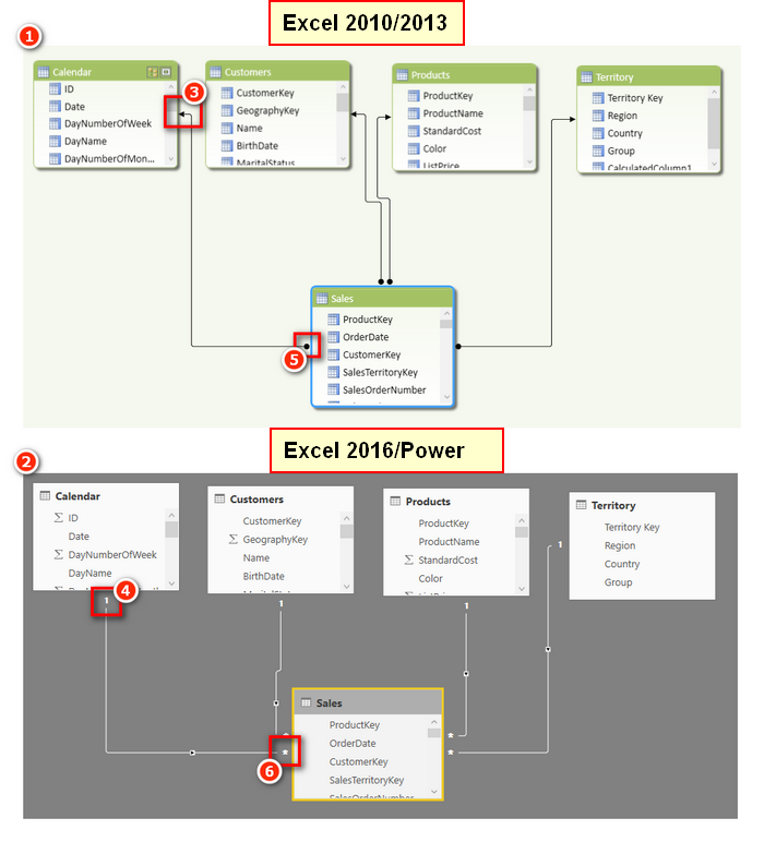
- Excel 2010 and 2013 have a different user experience in Diagram view compared to Excel 2016 and Power BI Desktop. You can see the differences between the different UIs in the image below. The earlier versions of Excel (see #1 below) have an arrow pointing to the “one” side of the relationship (#3) and a black dot on the “many” side (#5). Excel 2016 and Power BI have the new, improved UI (#2) with a 1 on the “one” side of the relationship (#4) and an * on the “many” side (#6).
Excel 2013
- In Excel 2013, the term calculated fields is used instead of measures. This was an unfortunate change made in Excel 2013 that lasted for this one version of Excel only, fortunately.
Excel 2010
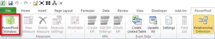
- The ribbon in Excel 2010 is slightly different in that it has a Power Pivot Window option (as shown below) instead of Manage in the later versions of Excel. The Power Pivot icon is the same in all Excel versions.
- Excel 2010 is the only version that uses a completely separate add-in to deploy Power Pivot, and this means there are two completely different field lists for pivot tables. The first time you stumble on the traditional PivotTable field list, you may be confused about what is happening, so being forewarned is forearmed. In the image below, note the different titles in the two different field lists. The one on the left (see #1 below) is the newer PowerPivot Field list; this is the one you should be using when working with Power Pivot. The one on the right (#2) is the original field list, and you don’t use it with Power Pivot pivot tables. But it is possible to have both open at the same time, and what is more confusing is that you can accidently open the wrong one without realising it. The key visual clues as to which one you have open are easy to spot: The titles are different, the PivotTable field list has special icons (#3), and the PowerPivot field list has a slicer drop zone (#4).

You Need Office Professional Plus
Not all versions of Excel come with Power Pivot as part of the offering. If you have the Home Edition or one of the many other lower-priced versions, you may be out of luck. And if you don’t have Power Pivot with your version of Excel, it is not something you can just upgrade to; you need to purchase a different version of Excel. If you have an Office 365 subscription, this will not be a major issue, but if you have a one-time purchase product, you will face a new expense to get a new version of Excel with Power Pivot.
Excel 2010
For Excel 2010 you can download the free Power Pivot add-in from the Microsoft website. You can search using a browser for the download. Just make sure you find and install Service Pack 2. You should search for Power Pivot for Excel 2010 SP2.
Excel 2013/2016
For these newer versions of Excel, you need to purchase Microsoft Office ProPlus to be able to get the Power Pivot add-in. ProPlus is used by most large organisations that purchase an E3 licence. You can see a full list of the versions that have Power Pivot (and the ones that don’t) at http://xbi.com.au/versions.
Excel 2010/2013
Power Query is a free add-in that you can download from Microsoft. Just search for Power Query in a web browser. After installing you will have a new tab called Power Query.
Excel 2016
Power Query comes bundled with Excel 2016. You can find it on the Data tab, Get and Transform.
Migrating Data from Power BI to Excel
If you read this heading and got excited, then I am sorry to tell you that you cannot migrate a Power BI Desktop data model into Power Pivot for Excel. It is possible to migrate the other way, though (from Excel to Power BI), as shown below.
Don’t forget that it is possible to use Analyze in Excel to create a new Excel workbook that points to a Power BI workbook loaded to PowerBI.com. This feature does require a Power BI Pro licence, however.
Here’s How: Importing Excel Power Pivot Workbooks to Power BI Desktop
It is possible to import a Power Pivot data model from an Excel workbook into Power BI Desktop, along with all the data connections, relationships, and measures. Unfortunately, any reports you have created in Excel will not be migrated and will need to be re-created in Power BI.
Follow these steps to import a Power Pivot workbook from Excel into Power BI Desktop:
1. In Power BI Desktop, select File, New. This will open a new blank Power BI Desktop file.
2. Select File, Import, Excel Workbook Contents.
3. Navigate to the Excel workbook you want to migrate, select it, click OK, and then select Import.
4. When you get the choice to copy the data from your queries or keep the connection (shown below), click Keep Connection.
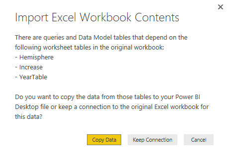
Note: Power BI Desktop doesn’t include the concept of linked tables. When you import an Excel workbook that contains linked tables into Power BI Desktop, you can either bring the data in as a one-off migration or retain the link to the original linked table in the original Excel workbook.
The Excel workbook data model is then imported into Power BI Desktop. From there you can proceed to use Power BI Desktop instead of Excel and build your own visualisations on top of the Power Pivot data model.
There are three places you can write DAX measures in Excel:
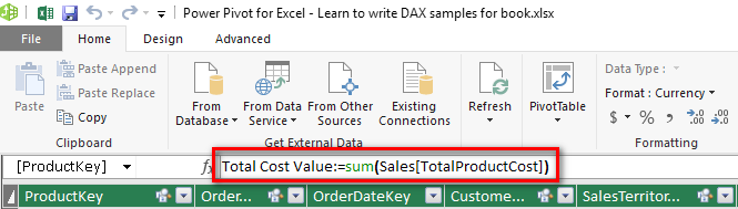
- You can write a measure in the formula bar in the Power Pivot window, as shown below. If you use this method, you must specify the measure name followed by a colon and then the formula.
- You can write and edit measures in any empty cell in the calculation area at the bottom of the Power Pivot window, as shown below. You also need to add a colon when writing a measure here.

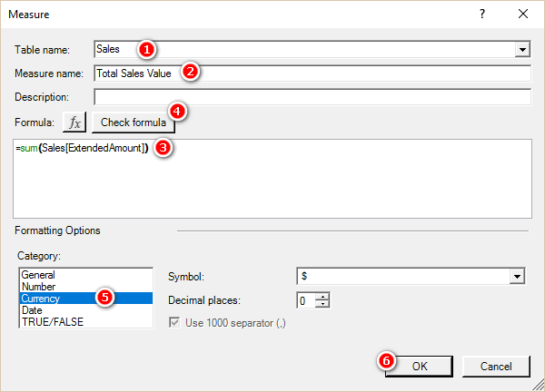
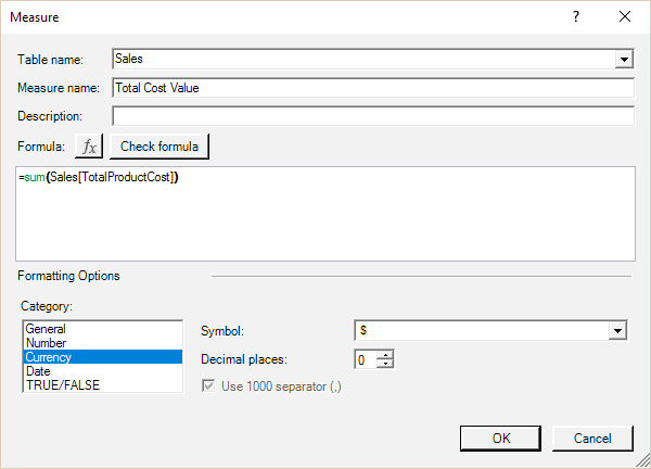
You can write measures in the Measure dialog in Excel, as shown below.
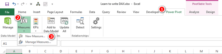
- You open this dialog in Excel by navigating to the Power Pivot tab (see #1 below) and selecting Measures (#2), New Measure (#3) or by right-clicking the Table name in the Pivot Table Fields list and choosing Add Measure….
Tip: In general, I recommend that Excel users write DAX in the Measure dialog box in Excel. I also recommend to first create a pivot table that provides some context for the measure you are about to write. If you do it this way, you will immediately see the measure appear in the pivot table once you click OK, and this will give you immediate feedback about whether the formula looks correct.
Note: At this writing, some versions of Excel 2016 do not automatically add a new measure to a pivot table as described in the tip above. However, Microsoft plans to reverse this change in a future update. Some older versions of Excel 2016 may therefore not automatically add the measure.
To create a new measure in Excel, follow these steps:
1. Create a new blank pivot table connected to your data model (or use an existing one if you already have something appropriate).
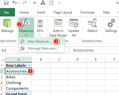
2. Add some relevant data to the rows in your pivot table (see #1 below).
3. Click inside the pivot table, navigate to the Power Pivot tab, click the Measures drop-down arrow (#2), and then select New Measure (#3). The Measure dialog appears.
Tip: You should use the Measure dialog shown below as a process flow/guide. If you don’t do this, you risk missing one or more of the steps. Missing a step will end up costing you time and causing rework. Get in the good habit of following the process steps I describe here, using the dialog to remind you of all the steps. Always follow the order outlined here.
4. In the Table Name drop-down (see #1 below), select the table where your measure will be stored.
5. In the Measure Name text box (#2), give the new measure a name.
6. In the Formula box (#3) write the DAX formula.
7. Click Check Formula (#4) to check whether the formula you wrote is syntactically correct. Fix any errors if you need to.
8. Select an appropriate formatting option from the Category list (#5), including a suitable symbol and decimal places in the area to the right of the Category list.
9. Click OK (#6) to save your measure.
Note: I generally don’t enter anything in the Description box, but it is there for you to use if you like. It’s for reference only and doesn’t impact the behaviour of the formulas.