4: DAX Topic: SUM(), COUNT(),
COUNTROWS(), MIN(), MAX(),
COUNTBLANK(), and DIVIDE()
This chapter starts out with some basic DAX formulas to get you started. Most of the DAX functions in this chapter accept a column as the only parameter, like this: =FORMULA(ColumnName). The exceptions are =COUNTROWS(Table), which takes a table (not a column) as the parameter, and DIVIDE(), which I cover later in the chapter.
All the functions in this chapter (except DIVIDE()) are aggregation functions, or aggregators. That is, they take inputs from a column or table and somehow aggregate the contents (differently for each formula).
Think about the column Sales[ExtendedAmount], which has more than 60,000 rows of data. You can’t simply put the entire column into a single cell in a matrix because Power BI can’t “fit” a column of 60,000 numbers into a single cell in the matrix.
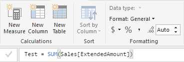
The following example shows a DAX formula that uses a “naked” column, without any aggregation function. This does not work when you’re writing a measure, as indicated by the error message.

You have to tell Power BI how to aggregate the data from this column so that it returns just a single value to each cell in the matrix. All the aggregators in this chapter effectively convert a column of values into a single value.
The correct way to write this measure is shown below.
Did you notice that this example uses the table name and the column name in the formula? Remember that this is best practice.
Note: Always refer to the table name and the column name when writing DAX. Never refer to a column without specifying the table name first. Power BI will do this for you automatically, but you can delete the table name manually (accidentally or deliberately)—though you should not do so! You will understand why I say this shortly.
Now IntelliSense Can Be Your Enemy, Too
It is worth mentioning at this point that sometimes IntelliSense can be your enemy. IntelliSense prompts you with a list of the available functions, tables, columns, and measures only if you are writing the formula correctly. This is very useful when you are doing it correctly because you get a list of the valid syntax. But the downside is that it can be confusing if you can’t see the list of possible functions, tables, columns, and measures that you are looking for and you don’t know why. If at any time when you are writing a formula you can’t see the functions, measures, columns, or tables you are looking for, you should stop and check your syntax. If the syntax is wrong, IntelliSense stops prompting you. Over time, you will learn to trust IntelliSense, and you will learn to stop and check when it is not working as you expect it to.
One important capability in DAX is that you can reuse measures when writing other measures. Say that you create a new measure called [Total Sales]. Once this measure exists in the Power BI data model, it can be referenced and reused inside other measures. For example, after creating the measure [Total Sales], you could use the following formula to create a new measure for 10% tax on the sale of goods:
Total Tax = [Total Sales] * 0.1
Note that the new measure [Total Tax] is a calculation based on the original measure [Total Sales] multiplied by 0.1.
It is good practice to reuse measures inside other measures.
Note: I did not add the table name in front of the measure name above. That is, I wrote [Total Sales] and not Sales[Total Sales]. Although you should always add the table name in front of a column (for example, Sales[ExtendedAmount]), it is best practice to omit the table name before a measure. The reason for doing it this way is that a reader can look at Sales[ExtendedAmount] and [Total Sales] and immediately tell that the first is a column and the second is a measure simply by the existence (or not) of the table name.
Writing DAX
It’s time to start to write some DAX of your own to get some practice. When I say write, I mean sit in front of your PC, open your workbook with the data from Chapter 1 loaded, and really write some DAX. Especially if you have never written formulas using these functions, you should physically do it now, as you read this section. Imagining yourself doing it in your mind is not enough.
If you haven’t already done so, go ahead and load the test data by following the steps in Chapter 1. Once it is loaded and prepared, you are ready to create the new measures in the following practice exercises. The first measure you will write is the same one from “Here’s How: Using IntelliSense” in Chapter 3.
Practice Exercises
Periodically throughout the rest of this book, you will find practice exercises that are designed to help you learn. You should complete each exercise as you get to it. The answers to all these practice exercises are provided in Appendix A.
Try to write DAX formulas for the following measures without looking back at how it was done. If you can’t do it, refer to Chapter 3 and then give it another go. Remember that you are here to practice! You can find the solutions to these practice exercises"Appendix A: Answers to Practice Exercises" on page 214.
Write DAX formulas for the following columns, using SUM().
1. [Total Sales]
You should have already written this measure earlier in this book. If not, write a new measure that is the total of the sales in the ExtendedAmount column from the Sales table.
2. [Total Cost]
Create a measure that is the sum of one of the cost columns in the Sales table. This measure uses exactly the same structure as the measure above, but it adds the cost of the product instead of the sales amount. You can use any of the product cost columns in the Sales table; all the cost columns are the same in this sample database.
3. [Total Margin $]
Create a new measure for the total margin, which is total sales minus total cost. Make sure you reuse the two measures you created above in this new measure.
4. [Total Margin %]
Create a new measure that now expresses the total margin from above as a percentage of total sales. Once again, reuse the measures you created above. I don’t cover the DIVIDE() function until later in this chapter, but you can try to work out how to use it by using the IntelliSense if you like.
5. [Total Sales Tax Paid]
Create another measure for total sales tax paid. Look for a tax column in the Sales table and add up the total for that column.
6. [Total Sales Including Tax]
The total sales amount above excludes tax, so you need to add two measures together to get this total.
7. [Total Order Quantity]
This is similar to the other measures, but this time you add up the quantities purchased. Look for the correct column in the Sales table.
How Did It Go?
As you worked through the practice exercises, did you do the following?
- Did you create a matrix first and put Products[Category] on Rows in your matrix? (Or did you put something else on Rows, as appropriate for these measures?) This is best practice because it enables you to you get feedback immediately after you write your measure; you can see the results.
- Did you right-click the Sales table and select New Measure to start the process? Doing so guarantees that the measure gets placed in the correct table, so you don’t lose it. Remember that you should always put a measure in the table where the data is stored, so these practice measures belong in the Sales table.
- Did you reference all columns in your measures in the format TableName[ColumnName] (i.e., always reference the table name)? Remember that you should never reference a column in DAX without first specifying the table name; always use the table name and the column name. Power BI makes this easy for you most of the time.
- Did you immediately apply formatting to your measure after you wrote it?
- Did you use the keyboard and look at the IntelliSense when you typed the measures? Try not to use the mouse. It may be faster for you now, but relying on the mouse will prevent you from getting faster with the keyboard in the future. Learn to use the keyboard and follow the process covered in “Here’s How: Using IntelliSense.”
Remember that the answers to all the exercises in this book "Appendix A: Answers to Practice Exercises" on page 214. Try to avoid peeking at the appendix when you should be thinking and typing. If you do the thinking now, you will learn how to do it, and that will pay you back in spades in the future.
Okay, it’s time to move on with a new DAX function.
As you write the formula shown below using COUNT(), take the time to look again at how IntelliSense can help you write DAX.
Remember that whenever you type a new formula, you can pause, and IntelliSense shows the syntax for and a description of the function. The description includes some very useful information. For example, in the figure below, the tooltip says that this function “counts the numbers in a column.” This gives you three very useful pieces of information. You’ve already worked out the first one: It counts. In addition, this tooltip tells you that the function counts numbers and also that the numbers need to be in a column. This should be enough information about the COUNT() function for you to write some measures using it.

Practice Exercises: COUNT()
Now it is time to write some DAX formulas using the COUNT() function. Find the solutions to these practice exercises in "Appendix A: Answers to Practice Exercises" on page 214.
Note: Don’t forget to set up a matrix before you work the following exercises. A good approach is to give the page in your last exercise a name, such as SUM, and then duplicate the page for this next exercise, giving it the name COUNT. This way, you can easily look back at your work later for a refresher. Whenever you set up a new matrix for a new exercise, make sure you have something meaningful on Rows, such as Products[Category]. Look at the image in “How Did It Go?” after these practice exercises if you are not sure how to set up the matrix.
8. [Total Number of Products]
Use the Products lookup table when writing this measure. Just count how many product numbers there are. Product numbers and product keys are the same thing in this example.
9. [Total Number of Customers]
Use the Customers lookup table. Again, just count the customer numbers. Customer numbers and customer keys are the same thing in this example.
How Did It Go?
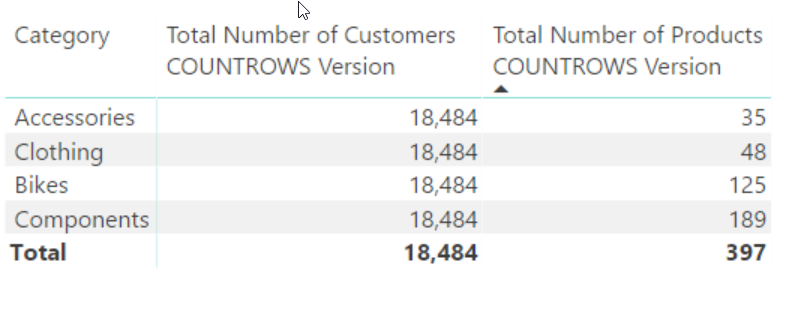
Did you end up with the following matrix?

If not, check your answers against those in"Appendix A: Answers to Practice Exercises" on page 214.
Note: The matrix above is a bit confusing because [Total Number of Customers] doesn’t seem to be correct. It is returning the same value for every row in the matrix, and this is not something you are used to seeing. But if you think about it, it actually does make sense. You are not counting how many customers purchased these product categories; you are counting the number of customers in the customer master table, and the number of customers doesn’t change based on the product categories; the customers are either in the master table or not. (You’ll learn more about this in Chapter 5.)
Did you get any errors that you weren’t expecting? Did you use the correct column(s) in your measures? Remember from the tooltip above that the COUNT() function counts numbers. It doesn’t count text fields, so if you try to count the names or descriptions, you get an error.
Let’s move on to a new function, COUNTROWS(). I prefer to use COUNTROWS() instead of COUNT(). It just seems more natural to me. These functions are not exactly the same, even though they can be used interchangeably at times. If you use COUNT() with TableName[ColumnName] and the column is missing a number in one of the rows (for some reason), then that row won’t get counted. COUNTROWS() counts every row in the table, regardless of whether all the columns have a value in every row. So be careful and make sure you select the best formula for the task at hand.
Practice Exercises: COUNTROWS()
For these exercises, rewrite the two measures from Practice Exercises 8 and 9 using COUNTROWS() instead of COUNT(). Find the solutions to these practice exercises in"Appendix A: Answers to Practice Exercises" on page 214.
10. [Total Number of Products COUNTROWS Version]
Count the number of products in the Products table, using the COUNTROWS() function.
11. [Total Number of Customers COUNTROWS Version]
Count the number of customers in the Customers table, using the COUNTROWS() function.
How Did It Go?
Not surprisingly, for Practice Exercises 10 and 11, you should get the same answer you got with COUNT(), as shown below.

You may have noticed that I sometimes use very long and descriptive names for measures. I encourage you to make measure names as long as they need to be to make it clear what the measures actually are. You will be grateful you did down the track, when you are trying to work out the fine difference between two similar-sounding measures.
Here’s How: Changing Display Names in Visuals
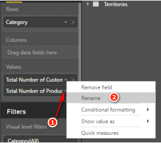
It is possible to change the display name of a measure or column once it is in a visual. Here are the steps:
1. Select the visual.
2. Find the measure or column in the Fields List Values section and click its down arrow (see #1 below).
3. Click Rename (#2). This renaming applies only to this single visual and does not change the actual name of the measure or column.
Here’s How: Word Wrapping in a Visual
Changing the measure name is useful when you want a shorter name to appear in your visual. Sometimes the name of a measure makes sense only in certain situations (i.e., in some visuals and not in other visuals). For such situations, if you want to keep using a longer descriptive name but want to make it fit in a matrix, you can turn on word wrap. To do so, follow these steps:
1. Make sure you have selected the matrix (see #1 below).
2. Navigate to the Format pane (#2).
3. Select Column Headers (#3).
4. Set Word Wrap to On by using the toggle (#4).
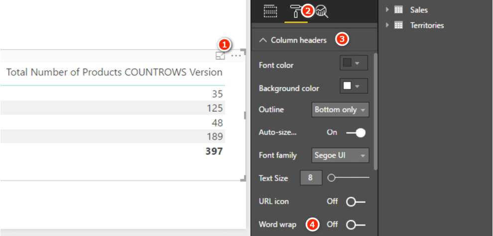
5. Wrap the columns by hovering your mouse to the right side of the column header in the matrix and then clicking and dragging the mouse to the left, as shown below.

6. The following image shows the result of applying word wrap to the matrix from earlier in this chapter.
DISTINCTCOUNT() counts each value in a column once and only once. If a value appears more than once in a column, it is still counted only once. Consider the Customers table. In this case, the customer key is unique, and by definition each customer key appears only once in the table. (Keep in mind that customer key = customer number.) So in this case, using DISTINCTCOUNT() with the customer key in the Customers table gives you the same answer as using COUNTROWS() with the Customers table. But if you were to use DISTINCTCOUNT() with the customer key in the Sales table, you would actually be counting the total number of customers that had ever purchased something—which is not the same thing.
Practice Exercises: DISTINCTCOUNT()
To practice using DISTINCTCOUNT(), create a new matrix and put Customers[Occupation] on Rows in the matrix and [Total Sales] on Values. Then write the following measures using DISTINCTCOUNT(). Find the solutions to these practice exercises in "Appendix A: Answers to Practice Exercises" on page 214.
12. [Total Customers in Database DISTINCTCOUNT Version]
You need to count a column of unique values in the Customers table. Go ahead and write the measure now. When you are done, add the [Total Number of Customers] measure you created earlier to the matrix as well. You should end up with a matrix like the one below.

How Did It Go?
Did you get the same answer as above in the new measure? Did you remember to format the measure to something practical (e.g., a whole number with thousands separators)?
13. [Count of Occupation]
Create a new matrix and put Customers[YearlyIncome] on Rows. Then create the measure [Count of Occupation].
Use DISTINCTCOUNT() to count the values in the Occupation column in the Customers table. You end up with a matrix like the one shown here. The way to read this matrix is that there are customers in three different occupations that have incomes of 10,000, there are customers across four occupations that have incomes of 30,000, etc.

Here’s How: Applying Conditional Formatting
It is much easier to read a matrix if you apply some of the formatting features that come with Power BI. For example, compare the matrix above left with the conditionally formatted version above right. I am sure you agree that it is much easier to gather insights from the version on the right. Follow these steps to apply this type of conditional formatting:
1. Make sure you have the matrix selected (see #1 below).
2. Go to the Format pane (#2), select Conditional Formatting (#3), and turn on the formatting effect you want to use, such as Data Bars (#4).

As you can see, using well-placed conditional formatting is a great way to make your matrixes easier to read and helps the insights jump out.
Practice Exercises: DISTINCTCOUNT(), Cont.
The following exercises give you more practice using DISTINCTCOUNT(). Find the solutions to these practice exercises in "Appendix A: Answers to Practice Exercises" on page 214.
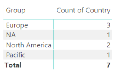
14. [Count of Country]
Create a new matrix and put Territories[Group] on Rows. Write a new measure called [Count of Country], using DISTINCTCOUNT() over the Country column in the Territories table. This matrix, as you can see below, shows you how many countries exist in each sales group.
15. [Total Customers That Have Purchased]
Create a new matrix and put Products[SubCategory] on Rows. Then, using DISTINCTCOUNT() on data from the Sales table, create the new measure [Total Customers That Have Purchased]. If you haven’t already done so, apply some conditional formatting to the matrix and then sort the column from largest to smallest (by clicking on the heading). You can see below that Tires and Tubes has the largest number of customers who have purchased at least once.

Here’s How: Drilling Through Rows in a Matrix
One of the features I really love about Power BI is the ability to nest columns and then drill through. Let’s look at how it works, using the matrix from above:
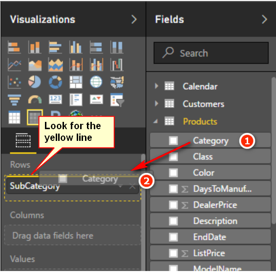
1. Make sure you have the matrix selected and then locate the Products[Category] column in the fields list (see #1 below).
2. Drag the column to the Rows drop zone (#2). Take care to check for the dotted yellow line, as indicated below. This line tells you where the column will be dropped (above or below the existing column).
3. Drop the Products[Category] column above the Products[SubCategory] column, as indicated by the arrow below.
4. Once you do this, the matrix changes in a few subtle ways, as shown below.
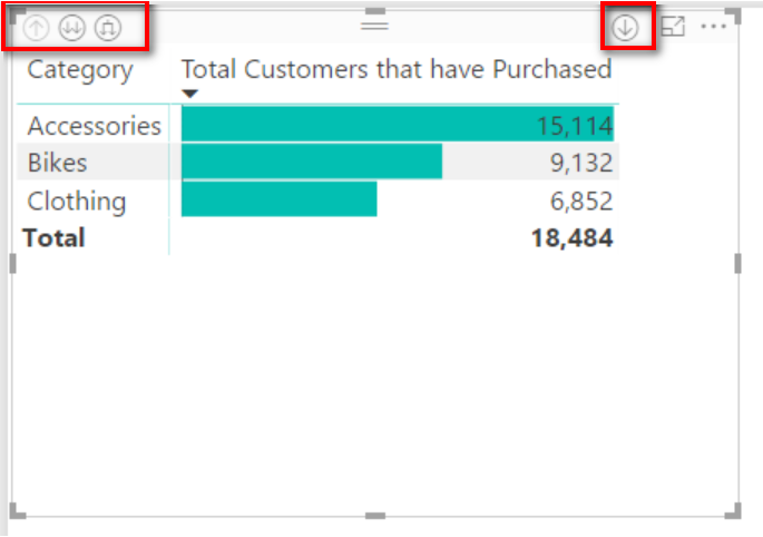
5. Note there are three new icons at the top left of the matrix, and there is one new icon at the top right. Also, if you right-click on a product category row (see #1 below), the submenu now has some new menu items.
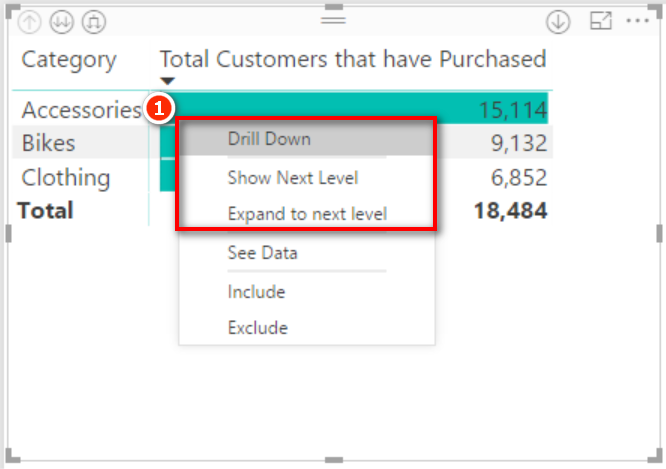
6. All of these menus provide drill-through capabilities for the columns you have added to the Rows drop zone in your matrix. Don’t get confused here; you add the columns from the tables to Rows in your matrix (by stacking one on top of another), and then you can drill through. Spend a few minutes trying out the various drill-through behaviours for each of these menus. You can drill down and drill up through the matrix.
7. Now put 'Calendar'[CalendarYear] on Columns in your matrix and notice how the matrix changes.
8. Go back to the conditional formatting settings for the matrix, turn off the data bars, and turn on colour scales. You should end up with a matrix like the one below. (I have used the Expand to Next Level drill-through feature in this matrix to get the nested layout shown below. This is very similar to how a pivot table looks.)

Tip: When you write these measures, remember to select the Sales table as the location to store them. Remember that best practice says to put a measure in the table where the data comes from. The easiest way to ensure that a measure is placed in the correct table is to start the process by first right-clicking the correct table and then selecting New Measure.
Practice Exercises: MAX(), MIN(), and AVERAGE()
MAX(), MIN(), and AVERAGE() are aggregators. They take multiple values in a column as an input and return a single value to the matrix. In these next practice exercises, you will create new measures using these aggregators. Find the solutions to these practice exercises in "Appendix A: Answers to Practice Exercises" on page 214.
You should use the columns of data in the Sales table for these exercises. There are some additional pricing columns in the Products table, but those prices are only theoretical prices, or “list prices.” In this sample data, the actual price information related to a transaction is stored in the Sales table.
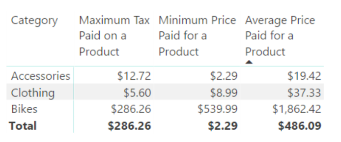
16. [Maximum Tax Paid on a Product]
Remember to use a suitable column from the Sales table and use the MAX() function.
17. [Minimum Price Paid for a Product]
Again, use a suitable column from the Sales table but this time use the MIN() function.
18. [Average Price Paid for a Product]
Again, use a suitable column from the Sales table but this time use the AVERAGE() function.
You should end up with a matrix like the one shown below.
Note: Notice that when you add these measures straight into a matrix, you get positive immediate feedback about whether your measures look correct. This is only a sense check, and you should of course confirm that your formulas are correct as part of the process.
Here’s How: Moving an Existing Measure to a Different Home Table
If you have been following my advice, when you create a new measure, you first right-click on the table where you want the measure to be placed, and then you select the new measure. However, even if you do it this way, it is possible at some stage that you will end up with a measure being in the wrong table. This is fairly easy to fix. Follow these steps to move a measure to a different table:
1. Locate the measure and select it. You can use the Search box at the top of the fields list, if necessary, to find the measure.
2. Navigate to the Modeling tab (see #1 below)
3. Select the Home Table drop-down list (#2) and select the correct table.

Practice Exercises: COUNTBLANK()
In the following exercises, you’ll use the COUNTBLANK() function to create a measure to check the completeness of the master data.
Create a new matrix and put Customers[Occupation] on Rows. Then start to write the new measure. In these exercises, you need to create measures to find out two things:
- How many customers are missing Address Line 2 from the master data?
- How many products in the Products table do not have a weight value stored in the master data?
Find the solutions to these practice exercises in "Appendix A: Answers to Practice Exercises" on page 214.
19. [Customers Without Address Line 2]
The AddressLine2 column is in the Customers table. As you write the measure [Customers Without Address Line 2], be sure you do the following:
4. Select the table where you want to store the measure and be sure to add it there.
5. Give the measure a suitable name.
6. Start typing the measure. Pause after you have started to type the formula and read the IntelliSense to see what the function does (if you don’t already know). As shown below, it does exactly what you want it to do: It counts how many blanks are in this column.

7. Complete the formula, apply the formatting, check the formula, and then save.
20. [Products Without Weight Values]
The column you need to use is in the Products table. You should end up with a matrix like the one shown below.

Note that the first measure, [Customers Without Address Line 2], is being filtered by the matrix (i.e., Customers[Occupation] on Rows), and the values in the matrix change with each row. But the second measure, [Products Without Weight Values], is not filtered; the values don’t change for each row in the matrix. You have seen this earlier in this book. The technical term for filtering behaviour in Power BI is filter context. Chapter 5 provides a detailed explanation of what filter context is, and that will help you understand what is happening here and why.
DIVIDE() is a simple yet powerful function that is also known as “safe divide.” DIVIDE() protects you against divide-by-zero errors in your visuals. A matrix, by design, hides any rows or columns that have no data. If you get an error in a measure inside a matrix, it is possible that you will see lots of rows that you would otherwise not see, and you will possibly also see some error messages. The DIVIDE() function is specifically designed to solve this problem. If you use DIVIDE() instead of the slash operator (/) for division, DAX returns a blank where you would otherwise get a divide-by-zero error. Given that a matrix will filter out blank rows by default, a blank row is a much better option than an error.
The syntax is DIVIDE(numerator, denominator, optional-alternate-result). If you don’t specify the alternate result, a blank value is returned when there is a divide-by-zero error.
Practice Exercises: DIVIDE()
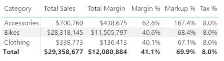
Create a new matrix and put Products[Category] on Rows. Then add [Total Sales] and [Total Margin $] to the matrix so you have some data to look at. This helps set the context for the new measures you will write next.
Write the following measures using DIVIDE(). Find the solutions to these practice exercises in "Appendix A: Answers to Practice Exercises" on page 214.
21. [Margin %]
Write a measure that calculates the percentage margin on sales (Total Margin $ divided by Total Sales). Reuse measures that you have already written.
Note: This is a duplicate of a measure, called [Total Margin %], that you wrote at the start of this chapter. This time, however, you write the formula by using the DIVIDE() function and give it the name [Margin %]. The result will be the same, of course.
22. [Markup %]
Find Total Margin $ divided by Total Cost.
23. [Tax %]
Divide the total tax by the total sales amount.
How Did It Go?
Did you format the last three measures as percentages, as shown below?