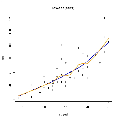
In this recipe, we will learn how to use lowess, which is a nonparametric model, and add the resulting prediction curve to a scatter plot.
For this recipe, we don't need to load any additional libraries. We just need to type the recipe in the R prompt or run it as a script.
First, let's create a simple scatter plot with the preloaded cars dataset and add a couple of lowess lines to it:
plot(cars, main = "lowess(cars)")
lines(lowess(cars), col = "blue")
lines(lowess(cars, f=0.3), col = "orange")

Standard R sessions include the lowess() function. It is a smoother that uses locally weighted polynomial regression. The first argument, in this instance, is a data frame called cars that gives the x and y variables (speed and dist). So we apply the lowess function to the cars dataset and in turn pass that result to the lines() function. The result of lowess is a list with components named x and y. The lines() function automatically detects this and uses the appropriate values to draw a smooth line through the scatter plot. The second smooth line has an additional argument, f, which is known as the smoother span. This gives us the proportion of points in the plot that influence the smoothening at each value. Larger values give us more smoothness. The default value is approximately 0.67, so when we change it to 0.3 we get a less smooth fit.