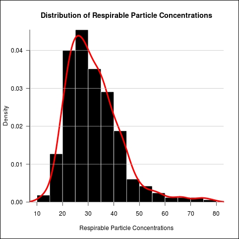
In this recipe, we will learn how to superimpose a kernel density line on top of a histogram.
We will continue using the airpollution.csv example dataset. You can simply type in the recipe code at the R prompt. If you wish to use the code later, you should save it as a script file. First, let's load the data file.
air<-read.csv("airpollution.csv")Let's overlay a line that shows the kernel density of respirable particle concentrations on top of a probability distribution histogram:
par(yaxs="i",las=1)
hist(air$Respirable.Particles,
prob=TRUE,col="black",border="white",
xlab="Respirable Particle Concentrations",
main="Distribution of Respirable Particle Concentrations")
box(bty="l")

lines(density(air$Respirable.Particles,na.rm=T),col="red",lwd=4)
grid(nx=NA,ny=NULL,lty=1,lwd=1,col="gray")

The code for the histogram itself is exactly the same as in the previous recipe. After making the hist() function call, we used the lines() function to plot the density line on top. We passed the result of the density() function call to the lines() function. The default kernel used is Gaussian, although other values can be specified. Take a look at the help file for density() for more details (run ?density at the R prompt).
To make the line prominent, we set its type to solid (lty=1), color to red (col="red"), and width to 4 (lwd=4).