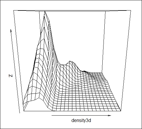
In this recipe, we will see how we can produce a three-dimensional visualization of a bivariate density plot. The two variables will represent two axes, and the estimated density will represent the third axis, which allows us to produce a three-dimensional visualization in turn.
For this recipe, we will use the airquality data from the datasets library. Particularly, we will use the Ozone and Temp variables:
attach(airquality)
We are required to call the MASS library in order to use the kde2d() bivariate kernel density estimation function:
library(MASS)
We are aiming to estimate the bivariate kernel density estimate and then visualize it. The estimation command is as follows:
# To fill the NA values in the variables and create new variable
# Create new ozone variable
Ozone_new <- Ozone

#Fill the NA with median
Ozone_new[is.na(Ozone_new)]<-median(Ozone,na.rm=T)

#Create new Temp variable
Temp_new <- Temp

#Fill the NA with median
Temp_new[is.na(Temp_new)]<- median(Temp,na.rm=T)
#Bivariate kernel density estimation with automatic bandwidth
density3d <- kde2d(Ozone_new,Temp_new)

#Visualize the density in 3D space
persp(density3d)

The steps involved in producing 3D density plot are as follows:
- Density estimation using the
kde2d()function. Within this function, the required arguments are the twoxandyvariables for which we want to estimate the density. Then, the bandwidthhcan be specified or it can be estimated automatically. We have used the default settings to estimate the bandwidth value. - Using the
persp()function to visualize the density in a 3D space. - The z axis represents the estimated probability density of the bivariate density function.