Process Design

3.1 Introduction to Process Design

Claus Thomy

The design of micro production processes and systems faces a variety of significant challenges today. This is due both to economic and to technological challenges. Generally speaking, in most industries micro production tends to be characterized by mass production, meaning very high lot sizes from several thousands (e.g. in medical technology) to literally billions (e.g. resistor end caps in the electronics industry). Moreover, such micro parts are often produced under severe cost pressure, with the market price for an individual part often being only a fraction of a € cent.

From an economic point of view, this means that the whole process chain has to be designed such that the output or production rate (e.g. measured in parts produced per minute) is maximized, whilst the defect rate (measured in ppm (parts per million) rejected) has to be minimized. From a technical point of view, these economic constraints are often very challenging, especially due to the specific characteristics of micro production with regard to materials, processes and products. Typical examples—in contrast to macro production—are a higher fragility of parts, scatter in and anisotropy of properties of the materials and parts produced, the highest tolerance requirements, and size effects.

In this context, and in order to deal with such challenges specific to micro production, an integrated “Micro-Process Planning and Analysis” (µ-ProPlAn) methodology and procedure with the required level of detail and complexity are suggested and implemented in software (Sect. 3.3). With this prototype software, the integrated planning of manufacturing, handling, and quality inspection at different levels of detail shall be enabled, reducing the overall effort and time for designing micro production processes, also pursuing a Simultaneous Engineering approach. Thus, three views with increasing levels of detail are provided: the process chain view, the material flow view, and the configuration view. The latter view is the closest to the part produced and the manufacturing process as such, and incorporates both qualitative and quantitative cause-effect networks to combine expert knowledge with statistical and learning-based data analysis methods. The challenge is that, between and within all views, complex interrelations occur, which are, for example, due to micro specific features such as high variances in properties. The µ-ProPlAn software prototype shall support process designers during all stages of planning from manufacturing process design to process configuration and the evaluation of process chain alternatives by analyzing and optimizing the underlying models, e.g. with respect to time- or cost-related parameters.

On a level closer to the actual micro manufacturing technology, in both bulk and sheet metal forming, the micro specific challenges illustrated above have to be dealt with, too (Sect. 3.2). In order to improve the planning especially of handling and assembly operations and systems, a micro specific enhancement of data exchange models on the basis of ISO 10303 is suggested. As handling of individual micro parts is fairly difficult, it is proposed and discussed to produce, convey and store these parts in the form of linked parts (either line-linked, ladder-linked or comb-linked). This reduces the effort for handling and storage (both long-term storage and highly dynamic buffering), but increases the effort for referencing parts with respect to their position and orientation at high production rates. Moreover, the force transfer especially during forming between neighboring parts due to low stiffness has to be considered, e.g. in the design of conveyors or (adaptive) guides, and can have an effect on part quality and accuracy. Understanding and modeling such scatter in accuracy can potentially allow us to widen the tolerance fields by methods such as selective assembly, thus minimizing waste. However, a prerequisite there is to master appropriate strategies for synchronization.

Acknowledgements The editors and authors of this book like to thank the Deutsche Forschungsgemeinschaft DFG (German Research Foundation) for the financial support of the SFB 747 “Mikrokaltumformen – Prozesse, Charakerisierung, Optimierung” (Collaborative Research Center “Micro Cold Forming – Processes, Characterization, Optimization”). We also like to thank our members and project partners of the industrial working group as well as our international research partners for their successful cooperation.

3.2 Linked Parts for Micro Cold Forming Process Chains

Philipp Wilhelmi*, Ann-Kathrin Onken, Christian Schenck, Bernd Kuhfuss and Kirsten Tracht

Abstract The method of production as linked parts allows a significant increase of output rates compared to the production of loose micro parts. In the macro range, it is already applied to sheet metal forming, for example, in the production of structural parts in the automobile or aviation industry, but a simple downscaling is not appropriate. The goal of producing high volumes of high-quality parts requires micro-specific methods. A holistic concept is presented considering planning and production. The main aspects of planning are the design of linked parts and the production planning. Furthermore, an approach is introduced to widen the tolerance field for assemblies to the production of linked micro parts. This approach requires the consideration of all affected process chains during planning. Linking of the parts enables them to be conveyed as a string and thereby simplifies handling, but also causes new challenges during production. Specific handling technologies are studied to overcome these challenges. Finally, a concept for the physical synchronization with regard to the investigation of tolerance field widening is presented.

Keywords Handling ∙ Assembly ∙ Production Planning

3.2.1 Introduction

Achieving high production rates is the key factor for a profitable industrial production of micro parts because of the typically low unit prices. Due to high tooling costs, this is especially relevant for cold forming. In addition to the small tolerances, fragility and sticking of the parts to each other or machine components make handling a major bottleneck in this context. This is mainly related to the surface-to-volume ratio, which increases with decreasing part size [Qin15]. The strength and weight of the parts depend on the volume, while the adhesion forces are related to the surface. Fantoni et al. have carried out extensive research in this field related to grasping [Fan14]. In the literature many different concepts for the handling of micro parts can be found, where grasping is involved at least for orientation or fixation, as presented in [Fle11], for example. However, most of these systems do not achieve the desired clock rates. Vibratory bowl feeders are the most common systems applied in the industrial environment so far [Kru09]. They are robust in their function and comparatively inexpensive, but only applicable for a limited range of types of micro parts and do not allow the production in fixed cycle times. The concept of production as linked parts, presented in [Kuh11], eliminates or strongly simplifies most of the speed-limiting handling operations like separation, grasping, releasing, orientation and fixation of individual parts. A linking structure keeps the parts interconnected and allows feeding of the parts as a string throughout the whole of the production stages. Examples of the industrial application of production as linked macro parts are mainly found in the manufacturing of sheet metal parts by punching, bending and deep drawing. The sheet is fed stepwise as a strip and processed by progressive dies. Lead frames for surface-mounted devices (SMD) or electrical connectors are produced as linked parts with features in the micro range. The sheet thickness for these applications is typically s ≥ 100 µm. In the MASMICRO project, the feeding and processing of thinner sheet material with progressive dies has been investigated [Qin08]. Merklein et al. considered a concept for massive forming as linked parts. Before the actual forming process, billets are formed from a metal strip (thickness: 1 mm ≤ s ≤ 3 mm) and remain therein [Mer12].

Until now, only single conceptual ideas were addressed. In the following, a holistic concept for the production planning and production of micro parts as linked parts is presented. This is done on the basis of two exemplary process chains illustrated in Fig. 3.1. The involved processes of deep drawing (see Sect. 4.2), laser rod melting (see Sect. 2.2) and rotary swaging (see Sect. 2.3) are considered in detail in the mentioned sections. Process chain 1 deals with ladder-linked parts, which are produced based on sheet material. Process chain 2 deals with the wire-based line-linked parts and involves massive forming. In addition to the single process chains, the synchronization of linked parts is included in the investigations.

../images/463048_1_En_3_Chapter/463048_1_En_3_Fig1_HTML.png — Fig. 3.1
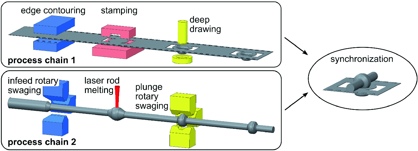
Considered process chains

In order to enable the mass production of different types of linked micro parts, two major fields of research are addressed. The first one is the planning of linked micro parts. In combination with the linking of the parts also micro-specific planning methods are required. The buffering of processes as well as the arrangement of the processes changes significantly, as shown in Sect. 3.2.2. The main focus of the second field of research is on the production of linked parts. Due to the linking of the parts, specific handling concepts are required. These are presented in Sect. 3.2.3 together with the synchronization of parts for building pre-assemblies.

3.2.2 Design and Production Planning of Linked Parts

The planning and controlling of processes is required to ensure an economic production. Considering the production of linked micro parts, the manufacturing and assembly of parts in high quantities and quality is influenced by the interconnection of the parts, the small dimensions, and low tolerances. Therefore, three subject areas are addressed in the following. In the first area, the design of the linked parts as well as a product model for deriving the data throughout the production stages are presented (see Sect. 3.2.2.1). These results are required for deciding which kinds of linked parts are applicable, and how to define the linking. Furthermore, the product model and the connection of processes are important for the second field of research. Due to the fact that every manufacturing stage influences the dimensions of workpieces in a different way and that the statistical distributions of the macro range are not applicable, micro-specific distributions are presented for the simulation of process chains, as well as recommendations for the arrangement of process steps for increasing the throughput (see Sect. 3.2.2.2). The third field involves the control of the production stages. In contrast to conventional approaches, the increase of assembled parts is reached by a design adjustment. The linking of the parts enables the consideration of trends occurring, for example, as caused by wear. The deviation of the geometrical properties is used for the identification of assemblies and for playing back this information to the design, as shown in Sect. 3.2.2.3.

3.2.2.1 Design and Product Model of Linked Parts

The design of linked parts is influenced by the production processes, and further functions that can be derived by the linking of parts. In general, the handling of parts in bulk requires functions like separation, orientation, positioning, and transfer [Kuh09]. In the case of micro parts, furthermore, scaling effects such as the dominance of adhesion forces increase the handling effort. The manufacturing and assembly as linked parts overcomes these size effects [Kuh11] and eliminates handling functions like the orientation of parts [Wek14a]. The transportation of each type of linked part differs in the flux of forces. The three basic types are line-linked parts, ladder-linked parts, and comb-linked parts. Line-linked parts are, for example, interconnected by the wire they are made of. An example of line-linked parts is shown in Fig. 3.2. Relevant design parameters for line-linked parts are the diameter of the spheres, the diameter of the wire, and the distance between parts.

../images/463048_1_En_3_Chapter/463048_1_En_3_Fig2_HTML.png — Fig. 3.2
Example of line-linked spheres

The flux of forces during transport of the linked parts runs through the parts themselves. The ladder-linked parts have a border area that is used for conveying the linked parts. The flux of forces does not run directly through the parts in this case. An example of ladder-linked parts are cups, which are left in the metal foil they are made of, as depicted in Fig. 3.3. Comb-linked parts are a hybrid type, where the flux of forces does not run through the parts themselves [Tra13].

../images/463048_1_En_3_Chapter/463048_1_En_3_Fig3_HTML.png — Fig. 3.3
Examples of the design of the border area of ladder-linked parts for absorbing forces

Besides the transfer of forces, such as the accelerating forces, the design of linked parts could be used for providing further functions and assisting while manufacturing parts. Especially the border areas of the ladder-linked parts could be utilized for this [Wek14]. Examples of the utilization of the border areas are lateral guide elements, pleats to increase the local stiffness, reference points, elements to modify the feeding force transmission in a belt conveyor, and spacers to protect the parts when they are coiled for storage [Kuh14]. Functional punching and elements in the rim of ladder-linked parts are depicted in Fig. 3.3.

The linked parts are produced in multistage processes. For this reason, product data models for a standard exchange of data are required. One possibility is the application of ISO 10303 STEP, which is the abbreviation of “Standard for the Exchange of Product Model Data”. Therefore, different methods, guidelines and application protocols are used. ISO 10303 is divided into classified series [ISO04]. Special areas are defined in the 200-series like the AP 207, where a product data model for sheet metal die planning and design is defined [ISO11]. Ladder-linked parts are made of sheet metal. For this reason, they are manufactured using sheet treating processes and could be integrated into AP 207 [Tra12].

Line-linked parts, on the other hand, have several requirements that are not covered by the AP 207. For this reason, a new application model, which covers the scope of micro forming is required. Therefore, the four steps of building an application activity model (AAM), developing an application reference model (ARM), mapping of the ARM, and developing an application interpreted model (AIM) have to be made [Wek16]. Regarding line-linked parts, interviews with researchers of the CRC 747 as process experts, and analysis of technical datasheets are used for identifying the required application objects [Tra12a]. An extract of this information is shown in Fig. 3.4 based on the example of line-linked parts.

../images/463048_1_En_3_Chapter/463048_1_En_3_Fig4_HTML.png — Fig. 3.4
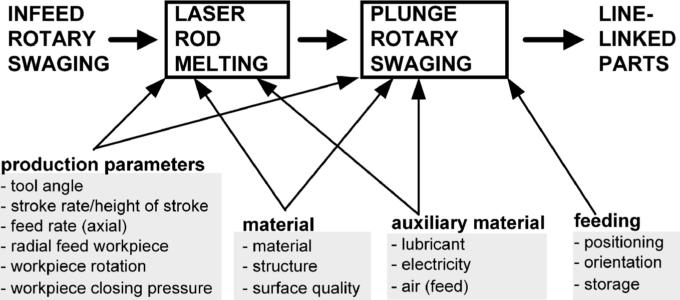
Information and data for plunge rotary swaging and laser melting

The identified application objects and their relation are the basis for the development of the AIM of the production process for linked parts. For completing the AIM, the geometry of the linked micro parts needs to be modularized. Therefore, it is especially important to summarize the piece part instances and the linkage parts instances [Wek16].

3.2.2.2 Production Planning

For achieving high output rates while guaranteeing an adequate part quality, it is important to profoundly understand the whole production process with its interfaces, technologies, and process conditions [Vol04]. In the following, important aspects for planning the mass production of linked micro parts are introduced, based on the example of manufacturing and assembling linked spherical parts and cups.

The occurrence of disturbances or scrap parts requires recommendations for actions that can improve multi-stage processes. Due to the fact that the impact of defects in shape, dimensions, and surfaces is much higher than in macro production [Wek14a], micro-specific process properties have to be taken into account. Simulation studies are an important tool in the planning of manufacturing lines even in the micro range. For reliable simulation results, it is important to use micro-specific distributions during the simulation of micro manufacturing processes. Therefore, micro-specific statistical distributions of ladder-linked parts [Wek13] and line-linked parts [Wek13a] are considered.

Looking at micro cups, the deviation of the rib thickness and the variability of the rib altitude, for example, are used for measuring the quality of the cups. Under consideration of the basic material, and the coating of the punching tool, the distributions for ladder-linked parts are investigated. In many cases, the burr distribution is applicable [Wek13].

For determining the statistical distribution of defects and changes in the geometry of line-linked parts, three different properties of line-linked parts are investigated as examples for distributions of micro parts. The first one is the diameter of the spherical preforms before processing by rotary swaging. The results show that, in total, 12% of the diameters of the preforms are not in the tolerated field. The second defect is the distance between the preforms. In total, 18% of the preforms are not in the tolerated distance. As the statistical distribution for the distance of preforms manufactured by laser rod melting, a Cauchy distribution is appropriate. The third quality criterion, which is especially important for further steps such as rotary swaging, is the volume of the parts. In this case, the Rayleigh distribution is appropriate for simulation of the parts properties. Furthermore, the results show that the volume of the produced parts more often exceeds the targeted volume [Wek13a]. Due to the fact that deviations of the shape, dimensions, and surfaces have a high impact on the production of micro parts, knowledge about these changing distributions is crucial for simulating processes. The simulation offers the possibility of analyzing different scenarios for the identification of appropriate places and capacities for buffering and discharging stations, as depicted in Fig. 3.5.

../images/463048_1_En_3_Chapter/463048_1_En_3_Fig5_HTML.png — Fig. 3.5
Simulation scenario of line-linked parts with and buffering and rejecting

Due to the rigid linking of the parts, the processing steps are also rigidly linked. Therefore, the configuration of buffers has a major influence on the throughput of the system and balances the varying process times. Furthermore, scrap parts are also present in the linked parts. Therefore, it is important to evaluate if the extraction of only one part or even a whole charge is to be recommended. Due to the fact that the unit prices are comparatively lower as in the macro range, it could be more profitable to extract charges [Wek14a].

The distribution and the amount of scrap parts influence the way in which the processes have to be arranged to improve the production of linked parts. In the following, recommendations for process chains are presented that are investigated by simulating the process chains of linked parts. In the case of a large amount of widespread scrap parts, it is best to extract only single parts instead of batches, due to the fact that there is a minor possibility of batches without defective parts. The implementation of buffers has a positive impact on the output, due to the balancing of the processes. Especially when scrap parts are extracted, it is important to buffer these processes. The decision whether defective parts should be extracted or manufactured in further steps is also dependent on the number of defective parts. When there is a large number of scrap parts, the extraction of the scrap parts has a positive impact on the throughput [Wek14a]. For a further increase of the number of assembled good parts, the geometrical deviations, which are caused by the whole manufacturing line, need to be considered. An approach to the widening of the tolerance field is presented in the following section.

3.2.2.3 Tolerance Field Widening

The linking of the parts maintains the production order. This facilitates an investigation of the deviation of geometrical dimensions over the production time. The knowledge of these deviations enables a widening of the tolerance field by identifying sections that could be assembled according to the fit [Onk17]. This approach is similar to selective assembly, where parts are sorted and matched for assembly according to their geometric characteristics. Several approaches to selective assembly, like the identification of assembly batches [Raj11], and reducing surplus parts using genetic algorithms [Kum07], are known. The adaptation of the production based on selective assembly has also been focused on in research. Approaches for selective and adaptive production systems offer the possibility of adjusting the process parameters directly during production. Kayasa et al. offer a simulation-based evaluation of adaptive and selective production systems [Kay12]. Lanza et al. provide a method for real-time optimization in selective and adaptive production systems [Lan15].

Due to the fact that the adaptation of processes is especially used in hard-to-control processes, the named approaches are not relevant for micro cold forming processes. A further contrast to these approaches is that the widening of the tolerance field enables a consideration of long sections of linked parts by using trends of geometrical deviations to identify matchable sections [Onk17]. This is applicable for two reasons. The first one is the sorted feeding by the interconnection of parts. Small tolerances for assembly are often caused by the required interchangeability of loose micro parts. Due to the retention of the production order, precise matching is feasible. The second reason is that in micro production, assemblies like valves, in the case of a defective component, are exchanged as a whole. Consequently, a widening of the tolerance field does not influence the interchangeability for maintenance or repair processes. For widening the tolerances, sequences of parts are matched under consideration of their fit. The methodology of widening the tolerance field is divided into three steps. The steps of clustering, matching and adjusting of the nominal value are performed after the production of the first batch, as shown in Fig. 3.6 on the basis of the example of cups and spheres [Onk17]. The results are used for the manufacturing and assembly of further batches. Within the first step, the trends are in focus. The consideration of the trend enables long sections that are matched in the second step [Onk17]. This is important for ensuring the mass production of further batches, due to the fact that a large number of interruptions for the changing of sections will reduce the productivity [Onk17a].

../images/463048_1_En_3_Chapter/463048_1_En_3_Fig6_HTML.png — Fig. 3.6
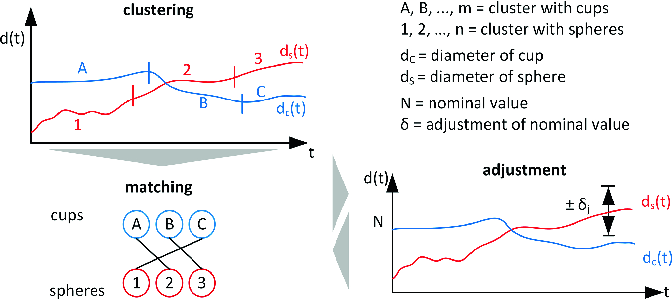
Schemata of the tolerance field widening

Linked parts clustering (LPC) is able to identify sections that are homogeneous according to the trends occurring. Essential for clustering trends is that the algorithm has to consider the linking of the parts. This could be performed by using cluster algorithms for networks. For building the clusters, similarity measures, which compare the characteristics of the parts, are used. This is important for considering the trends. The logic of the LPC is a basic configuration that could be adapted to the trend changes occurring using the assigning Factor (F). The algorithm is able to consider the linking of the parts and decides, on the basis of the Euclidian distance and F, whether the parts should be assigned to the present cluster or to a new one, as depicted in Fig. 3.7. The diameter of the parts is used for the calculation of the Euclidian distance [Tra18].

../images/463048_1_En_3_Chapter/463048_1_En_3_Fig7_HTML.png — Fig. 3.7
Linked parts clustering [Tra18]

In the second step, the parts are matched under consideration of the fit. Due to the fact that the matching of these two parts is similar to bipartite graphs, matching algorithms for bipartite graphs like the Munkres algorithm could be used [Onk17]. For the matching of clusters with varying lot sizes, these algorithms must be enhanced by adding additional rows due to the fact that most of them require N × N matrices.

As the third step of the tolerance field widening, the nominal value is adjusted. Due to the known development of the trends, an ideal nominal value can be identified. This means that the ratio of the two trends enables a large number of parts to be assembled. Therefore, after every adjustment of the nominal value, the number of pre-assemblies achieved is verified by another matching [Onk17]. The results of the tolerance field widening are influenced by the number of identified sections for matching and the trends occurring. Simulation results showed that with a larger number of sections also the number of mountable parts increases. The results emphasize that there is a point at which an explicit increase of sections only initializes a small increase of the number of pre-assemblies. Due to the fact that micro parts have a comparatively low unit price, such a small increase of assemblies is insignificant. Every interruption for changing sections leads to an increase of handling operations and thus decreases the throughput. The clock rates of the manufacturing and assembly of the parts are increased [Onk17a].

3.2.3 Automated Production of Linked Micro Parts

By applying the method of production as linked parts, on the one hand, time-critical sub-functions of the handling task like the grasping of individual parts and part orientation are avoided. On the other hand, by linking the parts, new challenges arise that must be dealt with to achieve the desired high output rates. The positioning in the processing zone cannot necessarily be considered independent of the transport. Processing may cause interactions and affect neighboring parts. Further, when applying the linked parts method to the production of assemblies, different process chains need to be synchronized. To ensure a stable material flow at high cycle rates and at the same time adequate precision for the positioning in the single production stages, specific equipment is necessary.

3.2.3.1 Handling Concept and Equipment

An approach for realizing a precise positioning in the macro range is to punch reference holes in the first production stage. In the following stages, pilot pins, which are integrated in the tools, realize a fine positioning. This approach, which is typically applied in the aforementioned example of production with progressive dies, hypothesizes that the general structure of the linked parts has a certain inherent stiffness and that it does not change during production. However, for the manufacturing of micro parts on the basis of thin sheet (h ≤ 100 µm) and for massive forming of line-linked parts, these requirements cannot be guaranteed. A further measure to simplify positioning, which is applied in the progressive dies, is the integration of all production stages into a compound tool. This allows low tolerances to be realized for the pitch between the single stages, which corresponds to the part distance a. In this way, a certain number of neighboring parts can be positioned and processed simultaneously. This is possible under the condition that all production stages have a similar character and can be actuated by a single press.

The proposed new approach references the parts with a sensor before positioning the processing zone. An example is illustrated in Fig. 3.8 by means of the investigated line-linked parts production. In production stage 1, preforms are generated by laser rod melting and consequently formed by rotary swaging in production stage 2. Without the referencing, a deviation from the desired distance a would lead to a positioning error in production stage 2.

../images/463048_1_En_3_Chapter/463048_1_En_3_Fig8_HTML.png — Fig. 3.8
Multi-stage production of linked parts

When supplying parts in bulk, the referencing of individual parts is a multi-dimensional problem. Besides the part position, the orientation of the part must be detected. Because of limitations in measuring rates as well as the processing power of the data evaluation hardware, this may present a bottleneck with regard to output rates. The linked parts approach reduces the problem to one dimension, which is a linear shift in the feed direction. This is valid under the assumption that, except for the feed direction, guides block all other degrees of freedom. In this case, a stationary sensor can be applied for referencing the linked parts during transport, as illustrated in Fig. 3.8. For that purpose, a position-dependent trigger signal is generated on the basis of the position sensor information of the conveyor. Each time the linked parts have moved a certain distance Δx_trigger, the sensor is triggered and acquires data. This approach was tested for three different measuring systems: an optical micrometer, a laser profile scanner and a line camera setup. The optical micrometer [Kuh12a] and the laser profile scanner [Kuh13] are both measuring systems based on image sensors and optimized for standard measuring tasks. They show quite good performances with respect to accuracy, but do not meet the requirements for the aspect of feed velocity. The approach of building up a measuring system on the basis of a camera in combination with suitable optics and illumination provides the best results in terms of both the accuracy and the possible feed velocities. By introducing an interpolation into the evaluation algorithm, the referencing is suitable for applications with output rates of more than 400 parts/min. This is valid even under the conservative assumptions of a part distance of Δx_part = 40 mm and a non-continuous conveyor. Both increase the resulting maximum feed velocity, which is v_feed,max = 1.6 m/s. Figure 3.9 illustrates the standard deviation of a measurement of the distance a between parts at different velocities compared to a reference measurement. The trigger distance was set to Δx_trigger = 50 µm in order to reach the desired cycle rate. For each velocity, eight linked parts (d_part ≈ 700 µm, l_part ≈ 1100 µm) were referenced and the seven distances between these parts were determined. The measurements were repeated ten times. The standard deviation is below 2.2 µm up to the targeted feed velocity of v_feed = 1.6 m/s. With higher feed velocity, the standard deviation increases noticeably [Wil17].

../images/463048_1_En_3_Chapter/463048_1_En_3_Fig9_HTML.png — Fig. 3.9
Standard deviation in dependency on velocity for part distance measurement with part referencing system (line camera), Δx_trigger = 50 µm

The sensor is ideally located close to the machining position, where the possible minimum distance depends on the actual machining process. Thereby, the applied conveyor must show an adequate positioning accuracy only for that limited feed distance. Two prototypes of conveyors were built and investigated during the experiments for the production of linked micro parts (see Fig. 3.10). One is a belt conveyor. The other conveyor works with two grippers, where one is stationary and the other is mounted on the slide of a linear axis, which is actuated by a linear motor.

../images/463048_1_En_3_Chapter/463048_1_En_3_Fig10_HTML.png — Fig. 3.10
Linked parts conveyors: a belt conveyor, b feed axis with grippers

Apart from the positioning accuracy of the conveyor, the linked parts influence the positioning. The low bending stiffness of the linked parts, which counts especially for thin sheet material, may lead to buckling and cause position deviations. In order to reduce this problem, the linked parts can be fed by pulling instead of pushing. Further, a tensioning of the linked parts with the help of a hysteresis brake or a second conveyor helps to solve this problem. Considering the accuracy of the feed axis with the grippers, small deviations are introduced as a result of the gripping. But, when assuming that after referencing no gripping is performed and the relevant part is directly positioned, the accuracy depends mainly on the feed axis and is in the sub-micrometer range. The belt conveyor has a large contact area between the linked parts and the coated belts. Thereby, high feed forces can be transmitted, and the local contact force may be reduced in order to avoid deformations. The rotational motion is converted by a friction power transmission in a linear feed. Consequently, different positional errors are introduced, for example, by conversion of the motion measurement from rotation to linear shift or the appearance of slip. Considering this, the feed axis shows a better performance in terms of positioning accuracy. Nevertheless, the belt conveyor can achieve a positioning accuracy in the lower micrometer range. One means of increasing the positioning accuracy is a direct measurement of the shift of the linked parts. Due to the fragility of the parts, contactless measurement is necessary. A sensor based on speckle correlation was investigated for that purpose and shows promising results, especially with regard to the achievable resolutions [Blo16].

Further, guides play an important role in the production as linked parts. Depending on the processes and their sequence, the guides along the process chain must fulfill different tasks. Besides the precise guiding of the linked parts transverse to the feed direction, they must isolate the individual processes from vibrations occurring in the other processes and damp the vibrations in the machining zones. Furthermore, compact size matters in order to enable the integration of the guides in the setups close to the machining zones. The guiding is particularly critical for line-linked parts, because of their longitudinally varying diameter. Hence, a concept for passive diameter adaptive guides for line-linked parts was developed [Wil17a]. The two variants illustrated in Fig. 3.11 were investigated under the aspects of guiding precision, suppression, and damping of radial vibrations as well as the influence on the feed force. Both variants were proven to enhance the guiding precision compared to non-adaptive guides. Further, they are suitable for suppressing the transmission of vibrations via the linked parts structure. Due to the material properties, the elastomer shows a better performance for damping vibrations in the machining zones. Nevertheless, form deviations of the linked parts from the desired geometry may result in inaccuracies for the guiding. The passive nature of the guides potentially introduces force peaks in the feed direction when a part passes through the guide. However, as they were experimentally determined to be below 0.1% of the applied feed forces, no negative effect is expected.

../images/463048_1_En_3_Chapter/463048_1_En_3_Fig11_HTML.png — Fig. 3.11
Adaptive guide concepts: a elastomer; b spring load, bearing balls

Finally, the automated production as linked parts demands specific storage. Two different types of storage are required: long-term storage after the production of parts and buffering between the manufacturing stages. The two types of storage differ mainly in their logistical properties, which are capacity and dynamic capabilities. Apart from that, the storage design depends on the linked parts’ geometrical properties (e.g. distance between parts, diameter and thickness) and mechanical properties (e.g. tensile strength, tolerable winding radius). Concepts for buffering are especially characterized by high process dynamics and low capacity. The linked parts could be buffered by extending the length of the conveyor line by using guide rollers as considered in [Rüc17]. Given that the required tensile stress is on the linked parts, guide rollers are arranged in line and the conveying line is minimal. The number of guide rollers defines the possible length of the buffer. For long-term storage, the well-known concepts of spooling and unspooling are suitable [Onk17]. These concepts are characterized by a high storage volume and a minor process flexibility. The line-linked parts are less sensitive to mechanical damage and can be stored in multiple paths and layers, and only the winding diameter is critical. Figure 3.12a illustrates line-linked parts on a spool. Spooling of ladder-linked parts is easier in one path only and with a protective layer in between, as depicted in Fig. 3.12b. This prohibits distortion of the ladder-linked parts caused by torsion. Furthermore, the insertion of the layer material prohibits the deformation and surface deformation of the sensitive parts [Rüc17].

../images/463048_1_En_3_Chapter/463048_1_En_3_Fig12_HTML.png — Fig. 3.12
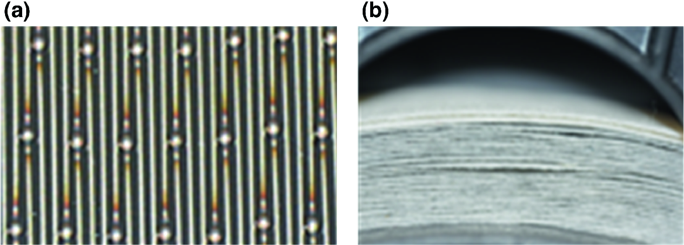
Storage of linked parts: a spooled line-linked parts, b ladder-linked parts spooled with protective layer

3.2.3.2 Effects Resulting from the Production as Linked Parts

There are different challenges that result from the linking of the parts. One is related to the fact that the feeder is applied for the transport, positioning and optional feeding during processing. Further, the structural connection leads to a transfer of forces between neighboring parts or the structure is changed by the processes. The concrete form of the effects that occur depends strongly on the manufacturing process applied.

For the production of line-linked preforms by laser rod melting (see Sect. 2.2), the applied conveyor is used both for the feeding during the process and for the transport afterwards. The requirements for these two tasks are different. Reaching the target position fast and a high stiffness against disturbing forces are the crucial points for the transport. For the laser rod melting, however, a good positioning behavior with respect to the desired feed velocity and a small overshoot is assumed to be favorable. The behavior of the conveyor and its effect on the production of preforms as linked parts was investigated experimentally [Wil18]. In the case of the control parameters, which are optimized for short transport times, the actual velocity of the investigated conveyor shows a significant deviation from the desired velocity especially for higher melting velocities. It could be shown that the process is relatively robust against such deviations. Further, an online adaptation of the control parameters can be applied as a countermeasure. The coupling of usually separate functions does not necessarily need to have an adverse effect. Rather, it could be proven that a further increase in the clock rate can be achieved by parallelization. Figure 3.13 illustrates the adapted process scheme for laser rod melting.

../images/463048_1_En_3_Chapter/463048_1_En_3_Fig13_HTML.png — Fig. 3.13
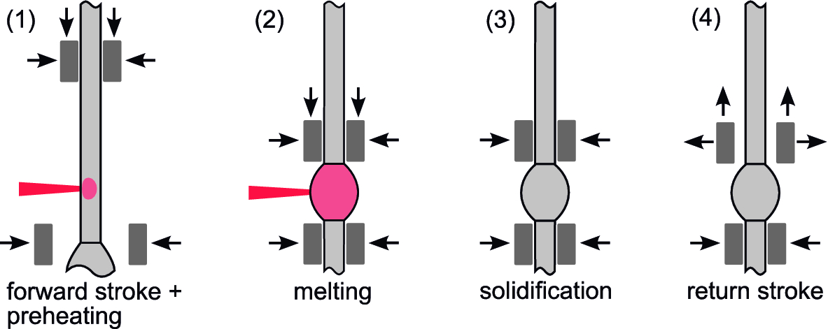
Process scheme of parallelized laser rod melting

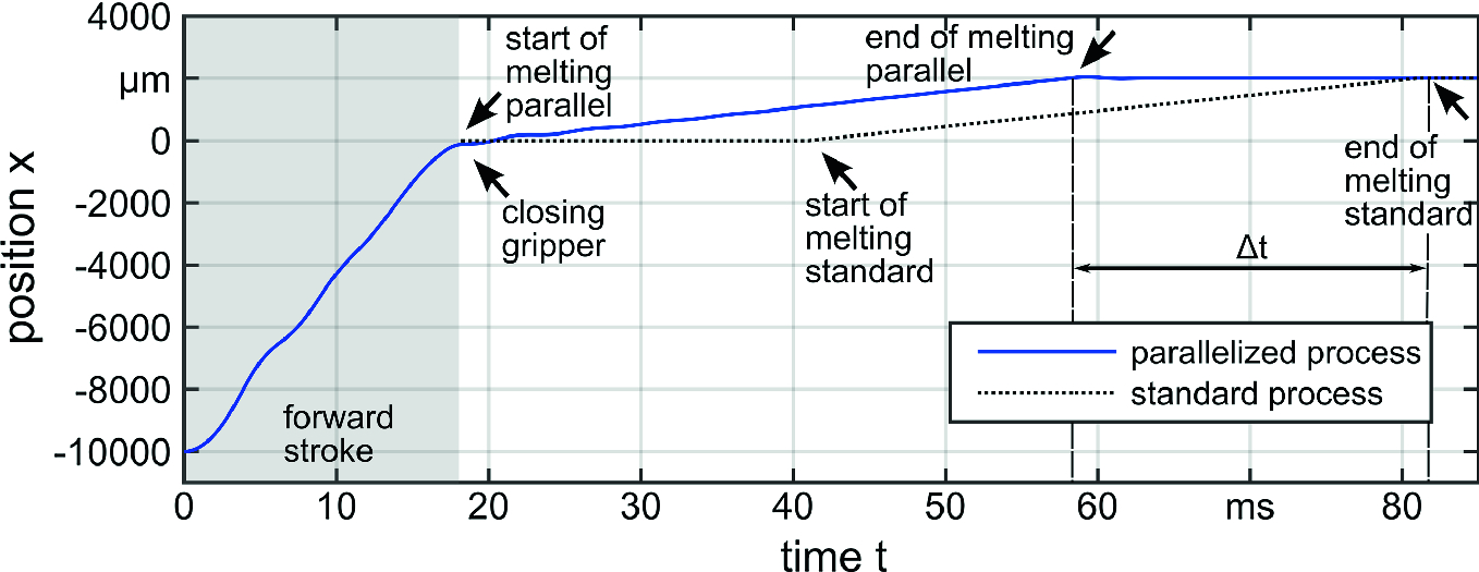
The preheating and the closing of the grippers are parallelized to the forward stroke. The effect of that adaptation on the cycle time is illustrated in Fig. 3.14, a measured position curve of the parallelized process. The transport motion is merged with the feed during melting. Thereby, the melting process can start earlier. In this example, the cycle time could be reduced by about 24 ms. The maximum cycle rate for laser rod melting of linked parts achieved with the described system is up to 300 parts/min. It is strongly influenced by the part volume and distance.

../images/463048_1_En_3_Chapter/463048_1_En_3_Fig14_HTML.png — Fig. 3.14
Position measurement of parallelized process

A change of the structure of the linked parts is especially observable in the case of massive forming. It has been found that the material flow during plunge rotary swaging leads to a significant elongation of the linked parts, which has a retroactive effect on the process. Assuming that the processed linked part is clamped on one side by the gripper of the conveyor and on the other side preloaded with a defined force, the behavior illustrated in Fig. 3.15 is observed. Before the processing, the linking structure is straight and the part is positioned in the center of the tool cavity. During processing, the part is centered within the cavity and the material flow leads to an elongation of the linking structure or wire on both sides of the part. Due to the low bending stiffness of the wire, this leads to buckling on the side of the conveyor and a spring force that presses the part against one side of the cavity within the tool. Thereby, inaccurate forming with asymmetric parts or even defects result [Wil15], as illustrated in Fig. 3.16. It could be shown that the effect on the part geometry can be more or less significant depending on the machine parameters. As shown in [Mou18], a convenient control of the applied forces or a compensation of the elongation improves the forming results and enables the production of symmetrical parts without defects.

../images/463048_1_En_3_Chapter/463048_1_En_3_Fig15_HTML.png — Fig. 3.15
Material flow during rotary swaging: a before processing, b during processing

../images/463048_1_En_3_Chapter/463048_1_En_3_Fig16_HTML.png — Fig. 3.16
Forming results: a bad part, b asymmetric part, c symmetric part

3.2.3.3 Synchronization of Linked Parts

In the here presented considerations related to synchronization, the main focus is not on the aspect of cycle rates. The key point is that individual linked parts of one type, or rather groups of linked parts of one type, are assigned to certain linked parts of a different type. This is particularly important for the already presented method of tolerance field widening. At the production level, synchronization means that assignment of the linked parts is performed physically in a way that simplifies the further handling. Instead of a direct assembly, also new types of linked parts can be created and form a pre-assembly. In that case, there are the three options [Onk18]:

directly joining both types of linked parts without separating them before;
separating the linked parts of both types and creating new linkage;
separating the linked parts of one type and joining them to the linked parts of the other type.

Option one is the direct joining of two types of linked parts without separation, which could cause problems in the further handling. An increased bending stiffness, for example, complicates winding. Comparing options two and three, the separation of only one type of linked part means less effort and therefore it is more convenient in most cases. For that reason, this option was investigated in an experimental setup. Figure 3.17 illustrates the basic function of the synchronization station. Both types of linked parts are referenced and positioned in the synchronization point. (The feed directions are indicated by arrows.) After that, they are welded via capacitor discharge welding in order to maintain the relative position and assignment between the synchronized parts for further handling. As the thin strip material is more sensitive to mechanical damage, the structure of the ladder-linked parts is kept and the line-linked parts are separated by mechanical shearing.

../images/463048_1_En_3_Chapter/463048_1_En_3_Fig17_HTML.png — Fig. 3.17
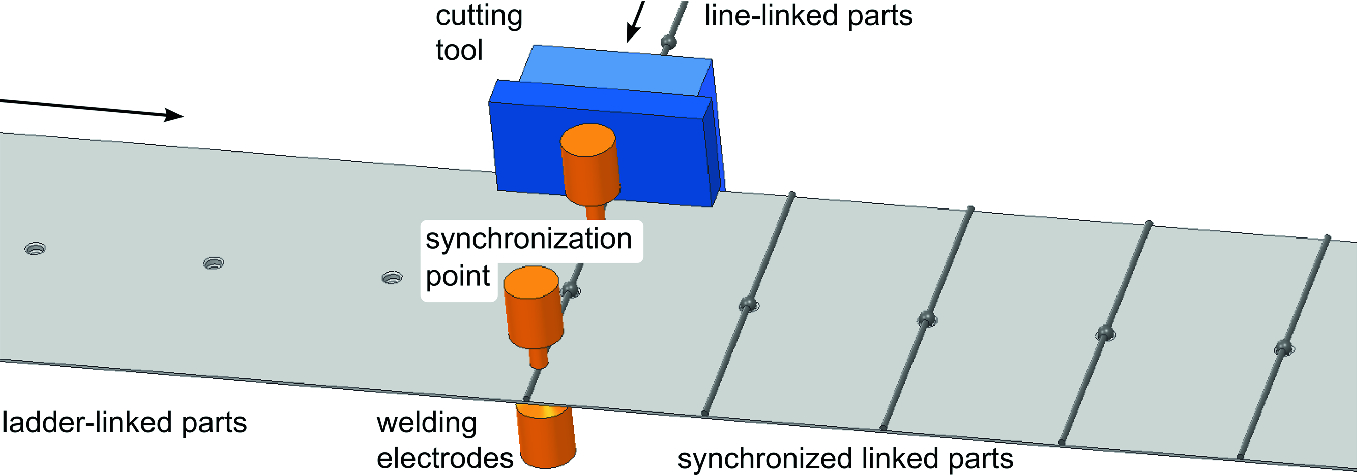
Basic function of the central module of the synchronization station

The complete setup is illustrated in Fig. 3.18. It requires all the previously presented handling technologies. The conveyor for positioning the ladder-linked parts is located on the left side of the central synchronization module. On the right side, another conveyor applies a constant force in order to tension the ladder-linked parts. The line-linked parts are fed orthogonally to the feed direction of the ladder-linked parts, from the back to the front. The sensors for the referencing are located in such a way that the linked parts are referenced close to the synchronization point. The central synchronization module includes a pneumatically actuated down holder, which fixes the linked parts after positioning and moves down the welding electrodes and the upper part of the cutting tool. The synchronization station is not only a concept for a possible synchronization setup, but also demonstrates the collaboration of the developed technologies in a practical scenario. It shows that, even with the inclusion of further technologies such as joining and cutting, clock rates of more than 200 parts/min can be achieved.

../images/463048_1_En_3_Chapter/463048_1_En_3_Fig18_HTML.png — Fig. 3.18
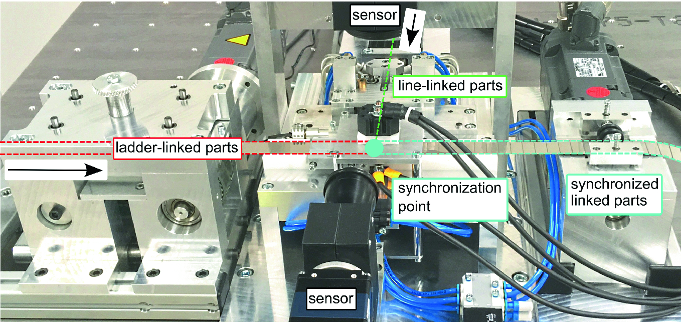
Complete setup—synchronization station

3.3 A Simultaneous Engineering Method for the Development of Process Chains in Micro Manufacturing

Daniel Rippel*, Michael Lütjen and Michael Freitag

Abstract The occurrence of size-effects requires detailed planning and configuration of process chains in micro manufacturing to ensure an economic industrial production. Existing methods lack the required level of detail and complexity as well as the handling of partly missing data and information, which is required for the micro domain. Consequently, this chapter describes a methodology for the planning and configuration of processes in micro manufacturing that aims to circumvent the mentioned drawbacks of the existing approaches. The methodology itself provides tools and methods to model, configure and evaluate process chains in micro manufacturing. Whereas the process design allows the detailed specification of micro manufacturing processes, the configuration is performed by the application of so-called cause–effect networks. Such cause–effect networks depict the interrelationships between processes, machines, tools and workpieces by relevant parameters. Thereby expert knowledge is combined with methods from statistics and artificial intelligence to cope with the influences of size-effects and other uncertain effects.

Keywords Modeling ∙ Production planning ∙ Predictive Model

3.3.1 Introduction

During the last decades, the demand for metallic micro parts has continuously increased. On the one hand, these components have become increasingly smaller while on the other hand, their shape complexity and their functionality are constantly increasing. Major factors contributing to this development are the increasing number and complexity of applications for micro components as well as the increasing demand for such components in the growing markets of medical and consumer electronics [Mou13]. Besides the growing demand for Micro-Electro-Mechanical-Systems (MEMS), which are generally produced using methods from the semi-conductor industry, the demand for metallic micromechanical components is growing similarly. These micromechanical components are used as connectors for MEMS, casings, or as contacts. They cannot be manufactured using semi-conductor technology and are usually produced by applying processes from the areas of micro forming, micro injection, micro milling etc. [Han06]. In this context, cold forming processes constitute an option for the economic mass production of metallic micromechanical components, as these processes generally provide high throughput rates at comparably low energy and waste costs [DeG03].

The efficient industrial production of such components usually requires high throughput rates of up to several hundred parts per minute [Flo14], whereby very small tolerances have to be achieved. These tolerances result from the components’ small geometrical dimensions, which, by definition, are below one millimeter in at least two dimensions [Gei01]. Additionally, so called size-effects can result in increasing uncertainties and unexpected process behaviors when processes, workpieces and tools originating from the macro domain are miniaturized [Vol08].

As a result, the planning and configuration of process chains is seen as a major factor of success for the industrial production of metallic micromechanical components [Afa12]. To cope with the occurrence of size-effects, companies require tools and methods for highly precise planning, covering the complete process chain. Thereby, they have to consider the interrelationships between processes, materials, tools and devices. In micro manufacturing, small variations in single parameters or characteristics can have a significant influence along the process chain and can finally impede the compliance with the respective tolerances [Rip14].

In order to facilitate the planning and configuration process, this chapter presents the “Micro-Processes Planning and Analysis” methodology which was designed to support process planners with a tool to plan and configure manufacturing process chains with the required level of detail. The methodology itself provides tools and methods to model, configure and evaluate process chains in micro manufacturing. Thereby, the configuration is performed by the application of so-called cause–effect networks, detailing the interrelationships between relevant process, machine, tool and workpiece parameters. These cause–effect networks combine expert knowledge with methods from the areas of statistics and artificial intelligence to cope with the influences of size-effects.

3.3.2 Process Planning in Micro Manufacturing

Within the literature, there are only very few approaches which allow the joint planning of process chains as well as the configuration of the processes involved. During the last few years, different articles have focused on the configuration of specific processes. Thereby, the configuration relies on detailed studies of the corresponding processes and is usually supported by very detailed physical models in the form of finite element simulations (e.g. [Afa12]). Another approach found in the literature focuses on the use of sample data (historical or experimental) as templates for the configuration of processes. Although these approaches enable a very precise configuration of a single process, the interrelations between different processes cannot be considered easily. Moreover, the construction of finite element simulations or the direct application of historical information requires a deep understanding of the processes, which is often unavailable due to size-effects or the novelty of processes.

Usually, classic methods like event-driven process chains, UML or simple flow charts are used in the context of process chain planning. Whereas these methods do not include the configuration of processes, Denkena et al. proposed an approach that indirectly addresses this topic [Den06]. This approach builds upon the modeling concept for process chains [Den11]. In this concept, a process chain consists of different process elements, again consisting of localized operations. These operations are interconnected by so-called technological interfaces that describe sets of pre- or post-conditions for each operation. While these interfaces can be configured manually, Denkena et al. also proposed the use of physical, numerical or empirical models to estimate the relationships between the pre- and post-conditions [Den06, Den14]. Although this approach enables configuration of the processes, the design of these models again requires very detailed insights into the processes. Moreover, within the micro domain, a single model can quickly be unsuitable to capture all relevant interrelations between process, machine, tool and workpiece parameters, particularly under the influence of size-effects, as its construction would require tremendous amounts of data.

3.3.3 Micro-Process Planning and Analysis (µ-ProPlAn)

The methodology “Micro-Process Planning and Analysis” (µ-ProPlAn) is being developed to support process designers in designing and configuring process chains (see [Rip17] for a more detailed description of the methodology). The modeling methodology µ-ProPlAn covers all phases from the process and material flow planning to the configuration and evaluation of these models [Rip14]. In this context, it enables the integrated planning of manufacturing, handling and quality inspection activities at different levels of detail. It consists of a modeling notation, a procedure model. and a set of methods and tools for the evaluation of the corresponding models. The evaluation covers methods to ensure the technical feasibility of the modeled process chains and production systems. Moreover, it includes a component to execute µ-ProPlAn models directly in terms of a material flow simulation to assess the modeled production system’s logistic performance.

The modeling notation consists of three views as depicted in Fig. 3.19, which represents different levels of detail. The first view focuses on the top-level process chains. This view’s notation closely follows the classic notation of process chains as described in [Den11]. Unlike the classical approach, process elements and operations are connected using process interfaces. In addition to the original technical parameters, these interfaces include logistic parameters. In an extension to the classical approach, operations act as interfaces to the next view. The material flow view further details operations by assigning those material flow objects used to conduct the operation (e.g. machines/devices, workpieces, tools, operating supplies or workers). This enables the modeling of specific production scenarios with specified resources and therefore allows an evaluation of the models regarding logistic aspects. For example, in the case of an existing production system, µ-ProPlAn can be used to assess the impact of new process chains (e.g. new products) on existing production plans or on the performance of the production system. Therefore, µ-ProPlAn offers the option to conduct material flow simulations based on the specified production system and the modeled process chains. This allows the early detection of e.g. bottlenecks or other undesired effects early during the planning stages. Consequently, it supports the selection of suitable resources, machines or devices for the new process chain. The third view focuses on the configuration of the processes and process chains using so-called cause–effect networks. These networks enable the evaluation of different process configurations (e.g. the use of different materials or different production speeds) and the assessment of the impacts of different choices on follow-up processes. As the cause–effect networks and material flow elements are closely connected, µ-ProPlAn reflects changes to the configuration of the material flow simulation and evaluates these e.g. regarding lead times, work-in-progress levels or the estimated product quality. Moreover, µ-ProPlAn provides several methods to evaluate the configured models. Besides the mentioned material flow simulation, the change propagation supports the process chain configuration and enables an estimation of a product’s intermediate and final characteristics.

../images/463048_1_En_3_Chapter/463048_1_En_3_Fig19_HTML.png — Fig. 3.19
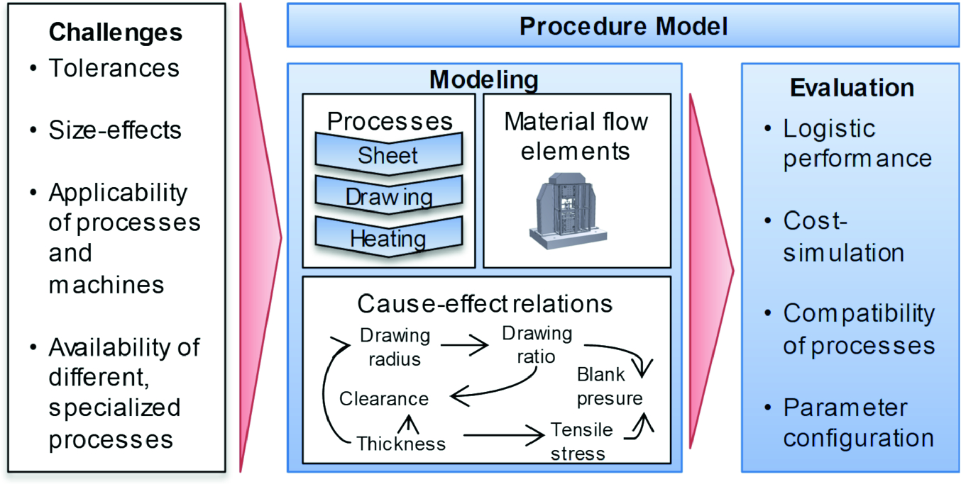
Components of the µ-ProPlAn Methodology [Sch13]

3.3.3.1 Modeling View: Process Chains

In general, process chains enable the structured modeling and planning of business processes, and depict the logic-temporal order of manufacturing, handling and quality inspection processes. Each process consists of one or more operations. Operations transform a set of input variables into output variables. These variables are called technological interfaces and describe the specific technical properties of the processed workpiece before and after each operation [Den11]. For example, a hardening operation modifies the variable hardness, which serves as an input and an output variable for the operation. On an aggregated level, processes provide and require similar technical interfaces with regard to other preceding or succeeding processes.

The notion of process chains provides an abstraction from material flow related resources and thus from specific manufacturing techniques. The hierarchical composition of the process chain enables the planning of the overall process chain based on processes and parameters relevant to the final product. In order to integrate the classic process chain models with the other views, the technological interfaces are extended to include logistic parameters, e.g. process durations or costs. Additionally, the operations themselves are extended to hold references of model elements from the material flow view, further detailing which devices and resources are involved in performing each single operation. At this, they directly provide the connection to the material flow modeling view.

3.3.3.2 Modeling View: Material Flow

The material flow modeling view consists of two parts. On the one hand, it is used to describe all the material flow elements within the considered system. On the other hand, it allows specific resources to be assigned to operations. Furthermore, it acts as an interface to the configuration or cause–effect view. Therefore, each material flow element is required to provide a minimal set of cause–effect parameters that differs depending on its type. During the evaluation, the material flow simulation uses these parameters to assess the logistic properties of the modeled system. Machines, tools, workers, operating supplies and workpieces constitute the major material flow elements. Table 3.1 summarizes the required parameters, which are necessary to estimate the logistic performance of the modeled system. Each operation requires at least one machine, a tool and a resulting workpiece. Additional resources can be assigned if applicable. During the machine definition, a setup matrix containing setup costs and durations has to be supplied.

Table 3.1

Mandatory parameters by resource (extended from [Rip14, Rip16])

Machines	Tools, workers, supplies	Operations
• Downtime on failure • Downtime on maintenance • Maintenance intervals • Setup times and costs • Mean time between failures • Costs while processing • Costs while idle	• Investment costs • (Tool) Service time in operations • (Worker) Costs while processing	• Duration • Probability of causing defect • Probability of detecting defect • Probability of falsely detecting defect

Machines

Tools, workers, supplies

Operations

• Downtime on failure

• Downtime on maintenance

• Maintenance intervals

• Setup times and costs

• Mean time between failures

• Costs while processing

• Costs while idle

• Investment costs

• (Tool) Service time in operations

• (Worker) Costs while processing

• Duration

• Probability of causing defect

• Probability of detecting defect

• Probability of falsely detecting defect

3.3.3.3 Modeling View: Configuration (Cause–Effect Networks)

To further detail each material flow element, µ-ProPlAn uses cause–effect networks, describing the interrelationships between relevant process parameters. Each network consists of a set of parameters and a set of cause–effect relationships, forming a directed graph. The set of parameters consists of all technical and logistic characteristics that are relevant to describe the object’s influence on the production process and at least consists of the parameters given in Table 3.1. In the case of workpieces, these include material properties, costs per piece or geometrical characteristics. As for production devices, these parameters include production speeds, forces or other characteristics that can be set, calculated or measured (see Fig. 3.20 for an example). From a modeling perspective, the cause–effect networks are hierarchical. Each material flow object (workpieces, machines, tools, workers, etc.) has its own cause–effect network, or at least a set of describing parameters. When combining these single elements into operations, process elements or process chains, higher-level cause–effect networks are created by describing additional relationships between the parameters of the networks or by connecting them to previously specified process interfaces (see Fig. 3.20).

../images/463048_1_En_3_Chapter/463048_1_En_3_Fig20_HTML.png — Fig. 3.20
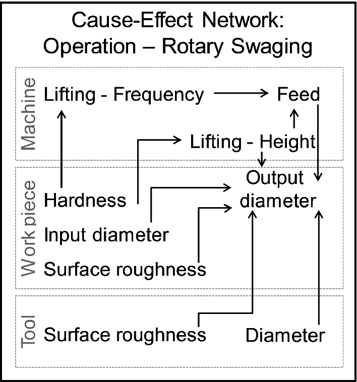
Hierarchy of cause–effect networks—Example of composition of a rotary swaging operation from the networks of the corresponding machine, tool and workpiece (after [Rip14a])

The design of cause–effect networks is divided into two steps: qualitative modeling and quantification. The qualitative model of the network is created by collecting all relevant parameters and denoting their influences among each other (see Fig. 3.20). Thereby, the process expert can facilitate the creation of the networks by pointing out the most relevant parameters and by indicating the relationships. Another option to attain a qualitative cause–effect network is the application of data mining techniques. For example, if experimental or production data are available, an analysis of this data can deliver preliminary insights into the cause–effect relations.

The second step concerns the quantification of the cause–effect networks. The objective is to enable the propagation of different parametrizations throughout the network. For example, this propagation allows the estimation of the outcome of processes for different materials or machining strategies. In Fig. 3.20, the use of a different material for the forging tool will result in a different surface roughness, thus influencing the overall output diameter of the processes. Through quantifying the cause–effect relationships, it is possible to estimate the results of parameter changes for all connected parameters along complete process chains.

3.3.3.4 Basic Quantification of Cause–Effect Networks

In the case of simple or well-known relations, µ-ProPlAn allows the implementation of mathematical functions to calculate a parameter’s value, based on its input parameters’ values. For example, a continuous manufacturing process will have a duration according to the total length of the workpiece divided by the selected feed velocity. More complex but well-established cause–effect relations could be included from the literature. Nevertheless, in the area of micro manufacturing, different parameters can have a more significant impact than in the macro domain, resulting in the inclusion of parameters that can usually be neglected. In addition, size-effects may induce a different behavior than usually observed. Therefore, it is often impossible to describe all the parameters and cause–effect relations comprehensively. As a result, µ-ProPlAn provides the capabilities to quantify cause–effect relations from experimental or production data by applying methods from the areas of data mining and statistics. Therefore, the qualitative cause–effect network is divided into a set of sub-problems. Each of these consists of one single dependent parameter and its independent parameters. To achieve a quantification, µ-ProPlAn utilizes a set of statistical regression or learning methods further detailed in Table 3.2. While statistical regression methods usually calculate a mathematical function to describe the expected value of the considered dependent variable, learning methods usually provide a more abstract model for a mean estimator (μ(x)). While these estimators can predict the value of the dependent variable, their models usually provide less insight into the mechanics behind the cause–effect relation and thus represent “black-box” models. Despite this disadvantage, they excel in their ability to learn arbitrary relations without prior knowledge of the relations shape (no prototype of the function has to be provided) and regardless of the problem’s dimensionality. In practice, the application of locally weighted linear regression (or interpolation) models has yielded good results in estimating complex relations.

Table 3.2

Regression and learning methods included in µ-ProPlAn [Rip14a]

Method	Description
Linear regression	As a fundamental multivariate regression function, µ-ProPlAn offers the option to perform a linear regression on the data provided. Additionally, µ-ProPlAn offers functionality to linearize e.g. exponential or logarithmic data
Polynomial regression	In the case of univariate cause–effect relations, a polynomial regression can be conducted
Tree/Rule regressions (e.g. [Hol99])	In contrast to the methods above, tree- or rule-based approaches do not result in a single analytic function. In general, they divide the search space into smaller segments for which a regression can be performed. Usually both methods use linear regressions for each segment
Locally weighted linear regression (LWL/LOESS) (e.g. [Fra03])	LWL constitutes an abstract prediction model, which performs a locally weighted linear regression each time a prediction is requested. Thereby, a kernel function is used to weight adjacent data points and finally a linear regression is performed. This method particularly excels in interpolating missing data in between available data points
Support vector regression(e.g. [Pla98])	Support vector machines are usually used as classifiers. Thereby, they learn models, which separate a set of data points into classes, maximizing the distance between each data point and the classification curve. The same method can be used for regression, particularly if the data provided contains strong variances
Artificial neural networks	A neural network usually consists of a number of layers, each containing a defined number of so-called perceptrons. The perceptrons of each layer are interconnected. During the supervised training of the network, these connections’ weights are adapted to recreate the desired output on the last layer

3.3.3.5 Characterization of Local Variances

While the application of the described methods enables the cause–effect networks to predict the estimated (mean) value of a parameter, they do not support the characterization and use of variances. Nevertheless, coping with these variances poses a major task for the configuration of process chains in micro manufacturing, in order to achieve a stable and efficient production. Moreover, the variance of a process can change for different parametrizations, requiring a localized approach. For example, when using a laser-chemical ablation process, the variance can change according to the flow rate of the chemicals. Therefore, µ-ProPlAn provides an estimated distribution as a prediction for a parameter’s value instead of a single mean value. Using these distributions, the process designer can e.g. try to select configurations with less variance, resulting in a more stable process/process chain, or assess the impact of less tolerated materials on the process chain.

Local calculation of the variance of each sampling point

In addition to the mean estimator, the local variance is computed for each point of the available sample data based on the corresponding standard deviation (σ). The method uses a set of experiments, each consisting of a number of independent variables (sampling points/configurations) x = (x₁, x₂,…) and a corresponding dependent variable (measurement). In the case of repeated measurements, each sampling point x corresponds to several values for the dependent variable, resulting in a vector y_x where the number of values |y_x| equals the number of measurements.

In a first step, the mean estimator μ(x) over all experiments is acquired using regression or learning techniques as described before. As a second step, the approach first determines a localized value for the standard deviation at each given point of sampling data and then further interpolates this information to enable a prediction of the variance for arbitrary points/configurations (σ(x)). The localized standard deviation for each sampling point is thereby calculated as usual, whereby the target vector y and the matrix source X^m×n, with n = |y| and m = |x|, are specifically constructed using a newly introduced parameter t to control the degree of locality. In general, the algorithm only tries to incorporate measurements for the single sampling point/configuration x. In cases where the number of repeated measurements y_x for x are insufficient (|y_x| < t), the algorithm incorporates additional sampling points into the calculation. On the one hand, small values for t ensure a very high locality, focusing on single sampling points or at least on very small areas around them. While a strong locality reduces the window size, it can negatively influence the estimation precision, as a precise estimation of the standard deviation requires a sufficient amount of data. On the other hand, a broader window size can usually yield better estimation results, while smoothing local changes in the standard deviation.

In the case of normally distributed values, this approach provides an accurate estimation of the overall standard deviation for each sampling point. Nevertheless, several practical applications require the estimation of skewed distributions. In this case, µ-ProPlAn estimates distinct standard deviations for both sides of the estimated mean value. Therefore, each vector of repeated measurements y_x is separated into two vectors, one containing all values smaller than the estimated mean value and the other containing all values greater than the estimated mean value for that given sampling point. The only exception are values that are equal to the estimated mean. If such a measurement is available within the data, its value is added to both vectors. Afterwards, the local standard deviation is calculated for each of these vectors as σ_Ui(x_i) and σ_Li(x_i). This separation enables the estimation of different standard deviations for both sides of the curve at the cost of precision. Due to the reduction of the available data points, the window size will inevitably increase, resulting in a stronger smoothing for each sampling point. The only option to counteract this would be the inclusion of additional repeated measurements.

Interpolation for arbitrary points and example

By applying the described local approach, µ-ProPlAn can characterize each of the provided sampling points by its mean and its estimated local standard deviation. In order to achieve an estimation of the standard deviations for arbitrary points, an interpolation takes place. Figure 3.21 depicts an example of an application of the local approach to a dataset containing 230 measurements of an ablation process. The dependent variable y depends on two independent variables x₁ and x₂. Figure 3.21a depicts the mean estimation obtained by using a locally weighted linear regression using an Epanechnikov kernel spanning approximately eight neighboring points. Figure 3.21b additionally depicts the estimated 95% probability intervals as green and red grids respectively, assuming the measurements were normally distributed.

../images/463048_1_En_3_Chapter/463048_1_En_3_Fig21_HTML.png — Fig. 3.21
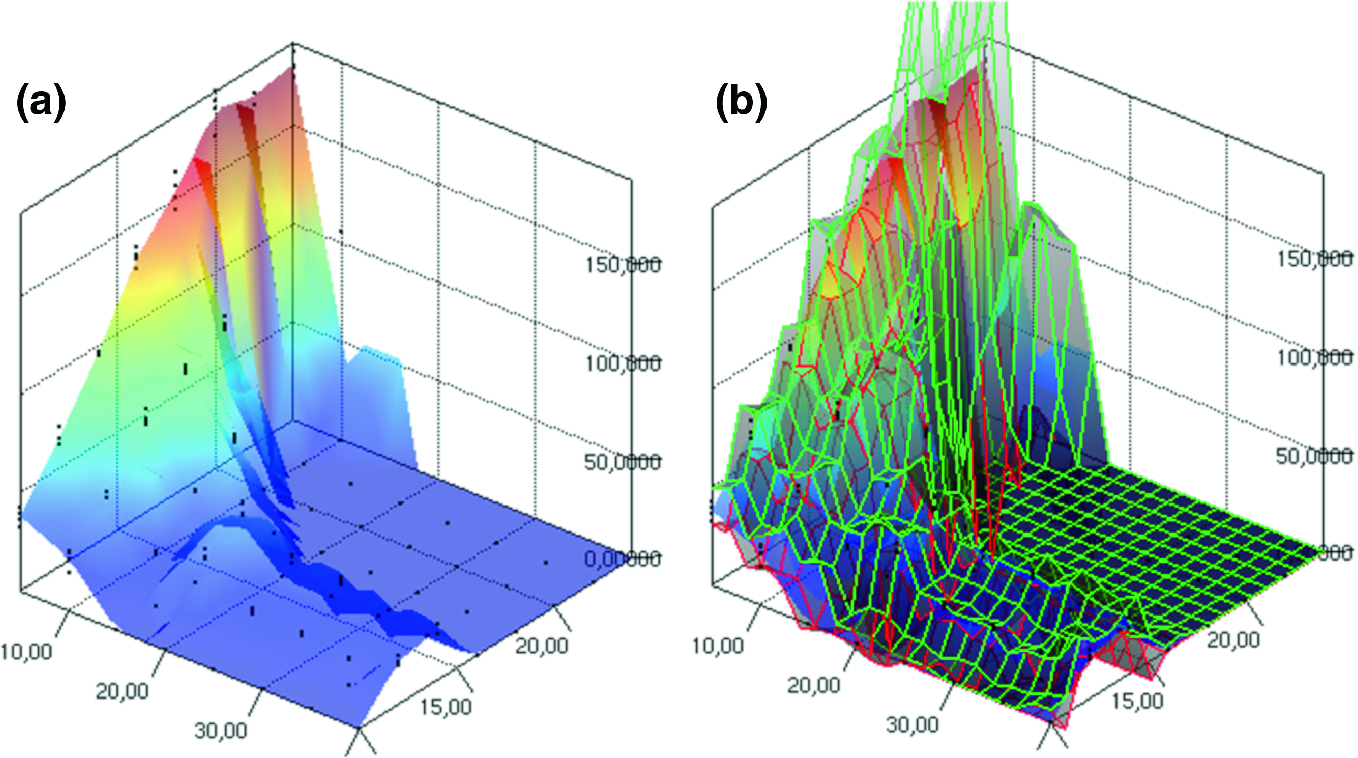
Example of application on a three-dimensional problem. a The heat-map colored surface depicts the mean estimator. b Additional green and red grids depict the 95% confidence interval

In general, µ-ProPlAn uses these standard deviations to describe the stability of a process in terms of its variance and its adherence to tolerances. In addition, it includes a technique to generate probability distributions based on these values. If only a single standard deviation was estimated, or if σ_Ui(x_i) and σ_Li(x_i) are close together, a normal distribution Ɲ(μ(x), σ(x)²) is generated. If they differ from each other, a Gumbel distribution is generated (also known as Extreme-Value Distribution). Therefore, a large number of sampling points is generated using two normal distributions derived as Ɲ_L(μ(x), σ_L(x)²) and Ɲ_U(μ(x), σ_U(x)²).

The resulting probability distributions can be used for further sampling, e.g. to calculate process capability indices c_p and c_pk. Therefore, µ-ProPlAn employs a Monte-Carlo simulation, whereby for a provided process configuration (e.g. materials, forces etc.) all dependent parameters along the process chain are sampled and, if appropriate, used as input for the remainder of the cause–effect network. By repeating this several times, the behavior of the overall process chain can be estimated in terms of e.g. quality-relevant target parameters like diameters or surface properties. The overall process capability indices are then calculated using Eqs. 3.1 and 3.2, with USL and LSL being the upper and lower specification limits according to the specified tolerances.

$C_{p} = \frac{USL - LSL}{6\sigma }$

(3.1)

$C_{pk} = \hbox{min} \left[ {\frac{USL - \mu }{3\sigma },\frac{\mu - LSL}{3\sigma }} \right]$

(3.2)

3.3.3.6 Simultaneous Engineering Procedure Model

To guide users through the process of model creation, a procedure model accompanies the methodology. This procedure model utilizes concepts of Simultaneous Engineering [Rip14]. In general, “Simultaneous Engineering describes an approach in which the different phases of new product development, from the first basic idea to the moment when the new product finally goes into production, are carried out in parallel.” [Sch02]. By parallelizing the development of the product and of the manufacturing processes, all characteristics and demands regarding the product’s complete life cycle can be taken into account early on. Ignoring such issues can lead to high costs in later stages of the product development or manufacturing [Pul11]. The application of Simultaneous Engineering techniques enables the early determination of these problems, which would usually only emerge during later stages of the production planning [Rei12].

The procedure model comprises three phases: process specification, configuration and analysis. The first two phases in particular should be conducted in parallel to the product development. Whenever the product design is extended or changed, these modifications should be integrated directly into the process chains.

The top-level process chain is designed during the process specification phase. First, the designer aligns all the required manufacturing processes with respect to the product design and defines the process interfaces. In a second step, the designer integrates quality inspection processes in between the manufacturing processes. As a last step of the specification, the designer integrates the required handling processes and operations. Some cases may require complex handling processes (e.g. the separation of single products or samples), while other cases can be satisfied by the integration of handling operations into existing processes. During the process configuration, suitable technologies for each process should be identified, as they determine or at least influence the process interfaces.

After defining the process chain and the according interfaces, the designer configures the processes. Based on the selection of technologies, he integrates relevant production parameters into the model and describes the parameters’ interdependencies (cause–effect relations). For each parameter, the designer specifies tolerances, which describe the range of allowed parameter values, in order to guarantee the required output values. In a second step, the parameters are set, thus describing concrete values for all production-relevant parameters in the process chain. By first specifying the tolerances, the designer is able to select resources according to the requirements of the process. Consequently, the process is aligned to the product’s quality requirements.

The last phase of the procedure is the analysis. Partially, it can occur in parallel to the specification of the material flow. Whenever a parameter is set to a specific value, the impact on the complete process chain can be analyzed according to the modeled cause–effect relations. As a result, the impact on later processes can be estimated and, if necessary, the designer can select other technologies or resources and adapt the model accordingly. In cases where no available technology is suitable to satisfy the product’s requirements, modifications to the product design or the development of new technologies can be addressed. Due to the proposed parallel development of the product and the design of the manufacturing process, such incompatibilities can be detected early on in the development process and higher costs can be prevented. In the last step of the analysis, technically feasible process chains can be simulated, using a material flow simulation, to determine their logistic performance and their behavior. The designer can compare different setups or processes and select the best option. In particular, if certain tools or workstations have to be purchased, the simulation can facilitate the decision between options [Sch08].

3.3.3.7 Geometry-Oriented Modelling of Process Chains

The geometry-oriented process chain design aims to provide an alternative way of modeling and designing process chains in µ-ProPlAn. The procedure model described before assumes a manual modeling and evaluation of each alternative chain. The geometry-oriented approach focuses on additional annotations to already modeled operations, in order to select and combine suitable processes. Thereby, each operation is annotated with information on the processes’ capabilities and limitations. In addition, workpieces can be specified by their geometrical features. Using a constraint-based search, suitable processes can be selected, combined and evaluated automatically. For these annotations, additional parameters are introduced to the cause–effect networks. These describe which geometries can be achieved by a process. Basically, µ-ProPlAn is adapted twofold. First, processes need to be annotated with their type (what they do). Second, each process requires the annotation of which geometrical features can be achieved under which circumstances.

The type of a process describes its function according to the standards DIN 8580 and VDI 2860. For manufacturing processes, the type describes if it is a (primary) forming process, a separating or joining process, if it is a coating process or if it just modifies the workpiece characteristics without changing the geometry. For handling processes, the type determines e.g. if it is a positioning or conveying process. Besides the definition of the type (optical, tactile, acoustic), quality inspection processes additionally require information on whether the process is in-line or destructive and about its resolution and measurement uncertainties.

The second adaptation describes the pre- and post-conditions of each process with respect to the geometrical features. Thereby, each process is annotated with a set of workpieces that can serve as input to the process, as well as a set of workpieces, which result from the process application to an input. In extension to the current model, each workpiece has a base geometry, describing e.g. if the workpiece is a sheet, a sphere, a wire etc. Each base geometry can be combined with additional base geometries to compose more complex workpieces. Figure 3.22, for example, shows a combination of a wire with a cone-shaped base geometry to represent a workpiece that could act as a plunger for a micro valve. Each base geometry can be assigned zero or more geometrical features like holes, steps, pockets or notches. These features and their parameters conform to the STEP-NC standard. Each of these features can again be assigned zero or more features on their own in a hierarchical manner.

../images/463048_1_En_3_Chapter/463048_1_En_3_Fig22_HTML.png — Fig. 3.22
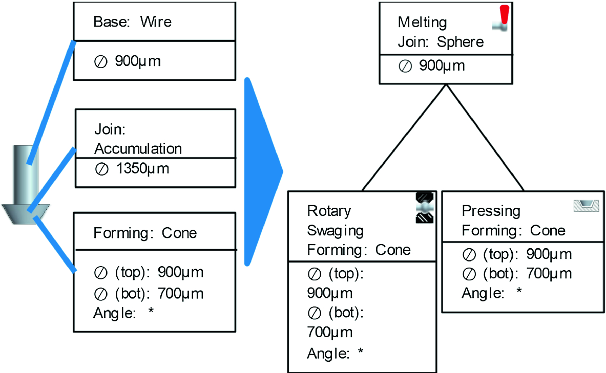
Example of the geometry based annotations and generated process chain alternative

By using these annotations, it becomes possible to apply constraint-based search algorithms to select suitable processes. During the modeling process, the designer specifies the hierarchical order of the base geometries and geometrical features required for the product. The software tool can search through all the stored processes within the model and select those that can achieve each feature. In the example in Fig. 3.22 there is only one alternative to join a sphere to a wire (melting). In contrast, there exist two alternatives to form this sphere into a cone. As the characteristics of each base geometry and each feature are expressed as parameters integrated into the processes’ cause–effect networks, the configuration of each alternative process chain can be performed in the usual way.

3.3.3.8 Analysis and Model Optimization

As mentioned before, µ-ProPlAn supports different methods to evaluate the process chain models using simulation-based and model-based evaluations. Technical characteristics (e.g. material or surface properties) or process capabilities can be estimated through the cause–effect networks, while logistic properties and the dynamic behavior of different alternatives can be estimated by transforming and simulating the different alternatives using the integrated discrete-event material flow simulation jasima [Hil12]. Using the respective results, the process designer can adapt the model and perform a manual optimization of different process chains, or compare different manufacturing scenarios. Nevertheless, a manual configuration of the processes can be time-consuming and prone to error. Therefore, µ-ProPlAn supports the configuration by providing methods to identify suitable values for input parameters, given a set of desired output values (e.g. for geometrical features) using meta-heuristics (i.e. a genetic search algorithm) and a pruned-depth first search algorithm. Both methods provide multiple settings, which are able to achieve the desired result within the specified tolerances. Moreover, Gralla et al. proposed a method to invert the cause–effect networks’ prediction models [Gra17] using techniques from the mathematical field of inverse modeling. The results show more reliable results in shorter times using these inverted cause–effect networks in combination with mathematical optimization techniques [Gra18].

The proposed methodology supports process designers during all stages from the manufacturing process design, the process configuration until the evaluation of process chain alternatives. In combination with the software prototype, it can be applied to different topics, e.g. for cost assessments of different configurations [Rip14], for the evaluation of different machining strategies [Rip14a], for the process characterization and configuration [Rip17b], or even as an abstraction for physics-based finite-element simulations to enable fast and precise process planning [Rip18a]. In addition, the methods underlying the cause–effect networks can easily be extended to utilize time-related information, thus enabling a re-training of cause–effect networks to cope with a lack of initial training data [Rip18] or in the context of predictive maintenance [Rip17a].

Open Access This chapter is licensed under the terms of the Creative Commons Attribution 4.0 International License (http://creativecommons.org/licenses/by/4.0/), which permits use, sharing, adaptation, distribution and reproduction in any medium or format, as long as you give appropriate credit to the original author(s) and the source, provide a link to the Creative Commons license and indicate if changes were made.

The images or other third party material in this chapter are included in the chapter's Creative Commons license, unless indicated otherwise in a credit line to the material. If material is not included in the chapter's Creative Commons license and your intended use is not permitted by statutory regulation or exceeds the permitted use, you will need to obtain permission directly from the copyright holder.

References

[Afa12] Afazov, S.M., Becker, A.A., Hyde, T.H.: Development of a finite element data exchange system for chain simulation of manufacturing processes. Adv. Eng. Softw. 47, 104–113 (2012)
[Blo16] Bloem, A., Wilhelmi, P., Schenck, C., Kuhfuss, B.: 2D position sensor based on speckle correlation—experimental setup for high-speed measurements and in field tests. In: Proceedings of 11th International Conference on Micro Manufacturing (ICOMM2016). Orange County, CA (USA), 29–31 March 2016, Paper# 17 (CD)
[DeG03] DeGarmo, E.P., Black, J.T., Kohser, R.A.: Materials and Processes in Manufacturing. Wiley (2003)
[Den06] Denkena, B., Rudzio, H., Brandes, A.: Methodology for dimensioning technological interfaces of manufacturing process chains. CIRP Ann. Manuf. Technol. 55(1), 497–500 (2006)
[Den11] Denkena, B., Tönshoff, H.K.: Prozessauslegung und -integration in die Prozesskette. In: Denkena, B., Tönshoff, H.K. (eds.) Spanen – Grundlagen, pp. 339–362. Springer, Heidelberg (2011)
[Den14] Denkena, B., Schmidt, J., Krüger, M.: Data mining approach for knowledge-based process planning. Procedia Technol. 15, 406–415 (2014)
[Fan14] Fantoni, G., Santochi, M., Dini, G., Tracht, K., Scholz-Reiter, B., Fleischer, J., Lien, T.K.: Grasping devices and methods in automated production processes. CIRP Ann. Manuf. Technol. 63(2), 679–701 (2014)
[Fle11] Fleischer, J., Herder, S., Leberle, U.: Automated supply of micro parts based on the micro slide conveying principle. CIRP Ann. Manuf. Technol. 60(1), 13–16 (2011)
[Flo14] Flosky, H., Vollertsen, F.: Wear behaviour in a combined micro blanking and deep drawing process. CIRP Ann. Manuf. Technol. 63(1) 281–284 (2014)
[Fra03] Frank, E., Hall, M., Pfahringer, B.: Locally weighted naive Bayes. In: 19th Conference on Uncertainty in Artificial Intelligence, pp. 249–256. Morgan Kaufmann (2003)
[Gei01] Geiger, M., et al.: Microforming. CIRP Ann. Manuf. Technol. 50(2), 445–462 (2001)
[Gra17] Gralla, P., et al.: Eine Methode zur Invertierung von Vorhersagemodellen in der Mikrofertigung. In: Vollertsen, F., et al. (eds.) 8. Kolloquium Mikroproduktion. BIAS Verlag, Bremen (2017)
[Gra18] Gralla, P., et al.: Inverting prediction models in micro production for process design. In: Vollertsen, F., et al. (eds.) MATEC Web of Conference, vol. 190. EDP Sciences, Les Ulis Cedex (2018). https://doi.org/10.1051/matecconf/201819015007Crossref
[Han06] Hansen, H.N., et al.: Dimensional micro and nano technology. CIRP Ann. 55(2), 721–734 (2006)
[Hil12] Hildebrandt, T.: Jasima-An Efficient Java Simulator for Manufacturing and Logistics. https://www.simplan.de/software/jasima/. Accessed 27 Sep 2018
[Hol99] Holmes, G., Hall, M., Frank, E.: Generating rule sets from model trees. In: 12th Australian Joint Conference on Artificial Intelligence, pp. 1–12. Springer, Heidelberg (1999)
[ISO11] International Organization on Standardization: ISO 10303-207: standard for the exchange of product model data—Industrial automation systems and integration—Product data representation and exchange. Part 207: Application protocol: sheet metal die planning and design
[ISO04] International Organization on Standardization: ISO 10303-11: standard for the exchange of product model data—Industrial automation systems and integration—Product data representation and exchange. Part 11: Description methods: the EXPRESS language reference manual
[Kay12] Kayasa, M.J., Hermann, C.: A simulation-based evaluation of selective and adaptive production systems (SAPS) supported by quality strategy in production. Procedia CIRP 3, 14–19 (2012)Crossref
[Kru09] Krüger, J., Lien, T.K., Verl, A.: Cooperation of human and machines in assembly lines. CIRP Ann. Manuf. Technol. 58, 628–646 (2009)Crossref
[Kuh14] Kuhfuss, B., Schenck, C., Wilhelmi, P., Langstädtler, L.: Electromagnetic linked micro part processing. In: Proceedings of 11th International Conference on Technology of Plasticity, ICTP 2014, 19–24 Oct 2014. Nagoya Congress Center, Nagoya, Japan. Procedia Engineering, vol. 81, pp. 2135–2140 (2014). https://doi.org/10.1016/j.proeng.2014.10.298Crossref
[Kuh13] Kuhfuss, B., Schenck, C., Wilhelmi, P.: Advanced laser profile scanner application for micro part detection. Laser metrology and machine performance. In: Proceedings of 10th International Conference on Laser Metrology, CMM and Machine Tool Performance (LAMDAMAP 2013), pp. 365–372. Euspen, Buckinghamshire, UK (2013)
[Kuh12a] Kuhfuss, B., Schenck, C., Wilhelmi, P.: Laser profile scanner application for micro part detection. Appl. Mech. Mater. 275-277, 2527–2530 (2013)
[Kuh11] Kuhfuss, B., Moumi, E., Tracht, K., Weikert, F., Vollertsen, F., Stephen, A.: Process chains in microforming technology using scaling effects. In: Menary, G. (ed.) International Conference on Material Forming (ESAFORM 2011), pp. 535–540. American Institute of Physics, Belfast, UK (2011) (online)
[Kuh09] Kuhfuss, B., Moumi, E.: Manufacturing of micro components by means of plunge rotary swaging. In: Proceedings of the Euspen International Conference, pp. 58–61 (2009)
[Kum07] Kumar, M.S., Kannan, S.M.: Optimum manufacturing tolerance to selective assembly technique for different assembly specifications by using genetic algorithm. Int. J. Adv. Manuf. Technol. 32, 591–598 (2007)Crossref
[Lan15] Lanza, G., Haefner, B., Kraemer, A.: Optimization of selective assembly and adaptive manufacturing by means of cyber-physical system based matching. CIRP Ann. Manuf. Technol. 64, 399–402 (2015)
[Mer12] Merklein, M., Stellin, T., Engel, T.: Experimental study of a full forward extrusion process from metal strip. Key Eng. Mater. 504-506, 587–592 (2012)
[Mou18] Moumi, E., Wilhelmi, P., Schenck, C., Herrmann, M., Kuhfuss, B.: Material flow control in plunge micro rotary swaging. In: Vollertsen, F., Dean, T.A., Qin, Y., Yuan, S.J. (eds.) 5th International Conference on New Forming Technology (ICNFT 2018), vol. 190, p. 15014. MATEC Web Conference (2018). https://doi.org/10.1051/matecconf/201819015014Crossref
[Mou13] Mounier, E., Bonnabel, A.: Press Release Emerging MEMS (2013). http://www.yole.fr/iso_upload/News/2013/PR_EmergingMEMS_August2013.pdf. Accessed 27 Sep 2018
[Onk18] Onken, A.-K., Wilhelmi, P., Tracht, K., Kuhfuss, B.: Increased output in micro production by tolerance field widening and synchronisation. In: Vollertsen, F., Dean, T.A., Qin, Y., Yuan, S.J. (eds.) 5th International Conference on New Forming Technology (ICNFT 2018), vol. 190, p. 15006. MATEC Web Conference (2018). https://doi.org/10.1051/matecconf/201819015006Crossref
[Onk17] Onken, A.-K., Rückert, P., Perl, C., Tracht, K.: Joining linked micro formed parts through tolerance field widening and synchronization. In: Schüppstuhl, T., Franke, J., Tracht, K. (eds.) Tagungsband des 2. Kongresses Montage Handhabung Industrieroboter (MHI2017). Springer, Heidelberg
[Onk17a] Onken, A.-K., Wilhelmi, P., Rückert, P., Tracht, K., Kuhfuss, B.: Toleranzfeldaufweitung durch gezielte Kombination von Fügepartnern in der Mikroproduktion. In: Vollertsen, F., Hopmann, C., Schulze, V., Wulfsberg, J. (eds.) Fachbeiträge 8. Kolloquium Mikroproduktion, pp. 259–266, 27–28 Nov 2017. BIAS Verlag, Bremen (2017) (in German)
[Pla98] Platt, J.: Fast training of support vector machines using sequential minimal optimization. In: Schoelkopf, B., Burges, C., Smola, A. (eds.) Advances in Kernel Methods—Support Vector Learning. MIT Press, Cambridge, MA (1998)
[Pul11] Pullan, T.T., Bhasi, M., Madhu, G.: Application of object-oriented framework on manufacturing domain. J. Manuf. Technol. Manag. 22(2), 906–928 (2011)
[Qin15] Qin, Y.: Micromanufacturing Engineering and Technology. William Andrew—Elsevier Science, Oxford (2015)
[Qin08] Qin, Y., Ma, Y., Harrison, C., Brockett, A., Zhou, M., Zhao, J., Law, F., Razali, A., Smith, R., Eguia, J.: Development of a new machine system for the forming of micro-sheet-products. Int. J. Mater. Form. 1 475–478 (2008)Crossref
[Raj11] Raj M.V., Sankar S.S., Ponnambalam S.G.: Minimizing clearance variations and surplus parts in multiple characteristic radial assembly through batch selective assembly. Int. J. Adv. Manuf. Technol. 57, 1199–1222 (2011)
[Rüc17] Rückert, P., Onken, A.-K., Tracht, K.: Beschädigungsfreies Speichern von Teileverbunden in der Mikroproduktion. In: Vollertsen, F., Hopmann, C., Schulze, V., Wulfsberg, J. (eds.) Fachbeiträge 8. Kolloquium Mikroproduktion, pp. 33–38, 27–28 Nov 2017. BIAS Verlag, Bremen (2017) (in German)
[Rei12] Reinhart, G., Meis, J.F.: Requirements management as a success factor for simultaneous engineering—enabling manufacturing competitiveness and economic sustainability. In: ElMaraghy, H.A., (ed.) Enabling Manufacturing Competitiveness and Economic Sustainability, pp. 221–226. Springer, Heidelberg (2012)
[Rip14] Rippel, D., Lütjen, M., Scholz-Reiter, B.: A framework for the quality-oriented design of micro manufacturing process chains. J. Manuf. Technol. Manag. 25(7), 1028–1049 (2014)Crossref
[Rip14a] Rippel, D., et al.: Application of stochastic regression for the configuration of a micro rotary swaging processes. Math. Probl. Eng. (2014) (article ID 360862)
[Rip16] Rippel, D., Lütjen, M., Freitag, M.: Geometrieorientierter Prozesskettenentwurf für die Mikrofertigung. Ind. 4.0 Manag. 32, 50–53 (2016)
[Rip17] Rippel, D., Lütjen, M., Freitag, M.: Local characterisation of variances for the planning and configuration of process chains in micro manufacturing. J. Manuf. Syst. 43(1), 79–87 (2017)Crossref
[Rip17a] Rippel, D., Lütjen, M., Freitag, M.: Simulation of maintenance activities for micro-manufacturing systems by use of predictive quality control charts. In: Chan, W.K.V., et al. (eds.) Proceedings of the 2017 Winter Simulation Conference, pp. 3780–3791 (2017)
[Rip17b] Rippel, D., et al.: Charakterisierung der Einflüsse einzelner Prozessparameter auf die Werkstückgeometrie beim Einstechrundkneten im Mikrobereich. In: Vollertsen, F., et al. (eds.) 8. Kolloquium Mikroproduktion, pp. 219–226. BIAS Verlag, Bremen (2017)
[Rip18] Rippel, D., Lütjen, M., Freitag, M.: Enhancing expert knowledge based cause-effect networks using continuous production data. Procedia Manuf. 24, 128–137 (2018)
[Rip18a] Rippel, D., et al.: Application of cause-effect-networks for the process planning in laser rod end melting. In: Vollertsen, F., et al. (eds.) MATEC Web of Conference, vol. 190. EDP Sciences, Les Ulis Cedex (2018). https://doi.org/10.1051/matecconf/201819015005Crossref
[Sch02] Schroeder, R.G., Flynn, B.B.: High Performance Manufacturing. Global Perspectives. Wiley, New York (2002)
[Sch08] Scholz-Reiter, B., Lütjen, M., Heger, J.: Integrated simulation method for investment decisions of micro production systems. Microsyst. Technol. 14(12), 2001–2005 (2008)
[Sch13] Scholz-Reiter, B., Rippel, D.: Eine Methode zum Design von Mikroprozessketten. Ind. 4.0 Manag. 29(2), 15–19 (2013)
[Tra18] Tracht, K., Onken, A.-K., Gralla, P., Emad, J.H., Kipry, N., Maaß, P.: Trend-specific clustering for micro mass production of linked parts. CIRP Ann. 67(1), 9–12 (2018)
[Tra13] Tracht, K., Weikert, F.: Handling of microparts. In: Vollertsen, F. (ed.) Micro Metal Forming, pp. 331–342. Springer, Heidelberg (2013)
[Tra12] Tracht, K., Weikert, F., Hanke, T.: Suitability of the ISO 10303-207 standard for product modeling of line-linked micro parts. In: Chryssolouris, G., Mourtzis, D. (eds.) 45th International Conference on Manufacturing Systems (CMS’2012), pp. 406–413. Athens (2012)
[Tra12a] Tracht, K., Weikert, F., Hanke, T.: Suitability of the ISO 10303-207 standard for product modeling of line-linked micro parts. Procedia CIRP 3, 358–363 (2012)Crossref
[Vol04] Vollertsen, F., Hu, Z., Schulze Niehoff H., Theiler, C.: State of the art in micro forming and investigations in micro deep drawing. J. Mater. Process. Technol. 151(1–3), 70–79 (2004)
[Vol08] Vollertsen, F.: Categories of size effects. Prod. Eng. 2(4), 377–383 (2008)
[Wek16] Weikert, F., Tracht, K.: STEP product model for micro formed linked parts. Prod. Eng. Res. Devel. 10, 293–303 (2016)Crossref
[Wek14] Weikert, F., Tracht, K.: Konstruktionsbaukasten für Leiterverbunde des Mikroumformens. Konstruktion 3 70–74 (2014) (in German)
[Wek14a] Weikert, F., Kröger, A., Tracht, K.: Auslegung von Prozessketten der Mikroumformung für die Verwendung von Teileverbunden. wt Werkstattstechnik online 104, 11/12, 722–727 (2014) (in German)
[Wek13] Weikert, F., Weyhausen, J., Tracht, K.: Statistical study for micro forming technologies used for linked parts production. In: Zaeh, M.F. (ed.) 5th International Conference on Changeable, Agile, Reconfigurable and Virtual Production (CARV’13), pp. 41–46. Munich, Germany (2013)
[Wek13a] Weikert, F., Weyhausen, J., Tracht, K., Moumi, E., Kuhfuss, B., Brüning, H., Vollertsen, F.: Beurteilung von Linienverbunden der Mikroumformung Tagungsband. In: Tutsch, R., (ed.) 6. Kolloquium Mikroproduktion. Shaker Verlag, Braunschweig (2013) (in German)
[Wil18] Wilhelmi, P., Schattmann, C., Schenck, C., Kuhfuss, B.: Interactions between feed system and process in production of preforms as linked micro parts. In: Vollertsen, F., Dean, T.A., Qin, Y., Yuan, S.J. (eds.) 5th International Conference on New Forming Technology (ICNFT 2018), vol. 190, p. 15014. MATEC Web Conference (2018). https://doi.org/10.1051/matecconf/201819015004Crossref
[Wil17] Wilhelmi, P., Schenck, C., Kuhfuss, B.: Linked micro parts referencing system. J. Mech. Eng. Autom. 7, 44–49 (2017). https://doi.org/10.17265/2159-5275/2017.01.006
[Wil17a] Wilhelmi, P., Schenck, C., Kuhfuss, B.: Handling in the production of wire-based linked micro parts. Micromachines 8, 169 (2017). https://doi.org/10.3390/mi8060169Crossref
[Wil15] Wilhelmi, P., Moumi, E., Schenck, C., Kuhfuss, B.: Werkstofffluss beim Mikrorundkneten im Linienverbund. In: Hopmann, Ch., Brecher, Ch., Dietzel, A., Drummer, D., Hanemann, T., Manske, E., Schomburg, W.K., Schulze, V., Ullrich, H., Vollertsen, F., Wulfsberg, J.-P. (eds.) Tagungsband 7. Kolloquium Mikroproduktion, pp. 31–38, Aachen, 16–17 Nov 2015. IKV, Aachen (2015). (CD) ISBN: 978-3-00-050-755-7

3. Process Design