5.1 Introduction to Quality Control and Characterization
Peter Maaß and Iwona Piotrowska-Kurczewski*
The increasing demand for miniaturization is having an immense impact on manufacturing technologies and is leading to the development of many novel and innovative production processes for high-precision micro parts. Industrially feasible micro production requires fast quality assurance control mechanisms, which need to take into account the micro-specific properties.
In this chapter several innovative technologies for quality control of production processes for high-precision micro parts will be presented. The proposed innovative solutions also address the need to ensure the quality of final products, which should be manufactured with approved (specified) materials and within certain performance requirements. Therefore, careful quality control is required during each production step.
Micro production processes and related techniques for quality control and characterization need to take into account the size effects that occur at the micro level, which lead to different scaling of forces and additional manufacturing errors that do not occur in macro processes. As a consequence, the conventional control methods for macro processes may fail, or become much more complicated or unreliable when applied to micro processes. In order to guarantee efficient quality assurance, possible error classes must be redefined and evaluated.
Moreover, in order to achieve an upscaling in the number of produced parts, the semi-finished products must be examined for mechanical properties. Micro production is characterized by a low aspect ratio of components to microstructure, which can dominate the mechanical behavior by means of the surface defects. It turns out that fatigue strength is an important component property.
This chapter presents some technical and methodological solutions for quality control and characterization measurement, with respect to size effects and up-scaling in micro production.
Digital holographic measuring systems (DHM) have the potential for complete (100%) and fast quality testing. Such a system is described in Sect. 5.2 together with fast algorithms for geometric evaluation and surface defect detection. The proposed method is demonstrated by inspecting cold formed micro cups.
This system is suitable for the automated examination and classification of micro deep drawn parts in an industrial environment. Together with automatic error detection, which uses the knowledge of the shape of the object, it allows the reliable inspection of components with a measuring speed of about one part per second. Further reduction of time is possible by additional optimization of the error detection algorithm. Section 5.3 shows the inspection of the interior of micro parts in the industrial environment.
To guarantee consistent production parameters for semi-finished products, which are subsequently used for the production of micro components, a characterization of their physical properties is of particular importance. Due to the often oligocrystalline character of these semi-finished products and components, it is necessary to use a suitable testing technique for static and dynamic investigations, as the mechanical properties are not transferable from the macroscopic point of view.
In addition, the micro semi-finished products and components often show inhomogeneities induced by the manufacturing process. On the one hand, these are directly reflected in the microstructure and on the other hand they have an effect on quantities such as hardness or residual stresses, which play a decisive role in the application. Mechanical testing, conventional metallography, SEM, EBSD, ultra-microhardness testing and X-ray residual stress analysis were used as measuring and analysis techniques suitable for the sub-millimeter range. In Sect. 5.4 the possibilities and limitations of two of these methods are illustrated using the example of mechanical testing and electron backscatter diffraction (EBSD).
Micro forming tools with high strength and hardness can be produced by means of laser chemical machining (LCM). The in situ geometry measurement of micro-structures during this process is based on the fluorescence of a liquid medium and principles of confocal microscopy. Section 5.5 focuses on that measurement technique, based on confocal fluorescence microscopy. It turns out that the model-based approach is suitable to detect the geometry parameter step height with an uncertainty of 8.8 μm for a step submerged in a fluid layer with a thickness of 2.3 mm.
Acknowledgements The editors and authors of this book like to thank the Deutsche Forschungsgemeinschaft DFG (German Research Foundation) for the financial support of the SFB 747 “Mikrokaltumformen—Prozesse, Charakerisierung, Optimierung” (Collaborative Research Center “Micro Cold Forming—Processes, Characterization, Optimization”). We also like to thank our members and project partners of the industrial working group as well as our international research partners for their successful cooperation.
5.2 Quality Inspection and Logistic Quality Assurance of Micro Technical Manufacturing Processes
Mostafa Agour*, Axel von Freyberg, Benjamin Staar, Claas Falldorf, Andreas Fischer, Michael Lütjen, Michael Freitag, Gert Goch and Ralf B. Bergmann
Abstract Quality inspection is an essential tool for quality assurance during production. In the microscopic domain, where the manufactured objects have a size of less than 1 mm in at least two dimensions, very often mass production takes place with high demands regarding the failure rate, as micro components generally form the basis for larger assemblies. Especially when it comes to safety-relevant parts, e.g. in the automobile or medical industry, a 100% quality inspection is mandatory. Here, we present a robust and precise metrology method comprised of a holographic contouring system with fast algorithms for geometric evaluation and surface defect detection that paves the way for inspecting cold formed micro parts in less than a second. Using a telecentric lens instead of a standard microscope objective, we compensate scaling effects and wave field curvature, which distort the reconstruction in digital holographic microscopy. To enhance the limited depth of focus of the microscope objective, depth information from different object layers is stitched together to yield 3D data of its complete geometry. The 3D data map is converted into a point cloud and processed by geometry and surface inspection. Thereby, the resulting point cloud data are automatically decomposed into geometric primitives in order to analyze geometric deviations. Additionally, the surface itself is checked for scratches and other defects by the use of convolutional neural networks. The developed machine learning algorithm makes it possible not only to distinguish between good and failed parts but also to show the defect area pixel-wise. The methods are demonstrated by quality inspection of cold formed micro cups. Defects larger than 2 μm laterally and 5 μm axially can be detected.
Keywords Digital holographic microscopy · Geometry · Surface defect
5.2.1 Introduction
Quality inspection is an essential tool for quality assurance during production. Generally, the precise geometrical and surface inspection of a test object plays a decisive role for developing and/or optimizing the manufacturing process. In the microscopic domain, where the manufactured objects have a size of less than 1 mm in at least two dimensions, very often mass production takes place with high demands regarding the failure rate, as micro components generally form the basis for larger assemblies. Especially when it comes to safety-relevant parts, e.g. in the automobile or medical industry, often a 100% quality inspection is mandatory [Kop13].
Achieving 100% quality inspection is especially challenging in the micro-domain, e.g. when measurement uncertainty has to be in the range of a few microns, as there is usually a trade-off between precision and speed [Ago17]. Processes like micro cold forming, however, allow for production rates of multiple parts per second [Flo14]. Presently, no solutions exist that are fast, precise and suitable for in-process measurements at the same time [Ago17b]. Actually, most industrial quality inspection processes of micro parts rely on manual sampling using confocal microscopy. This means also that no automatic data processing regarding the geometry and surface inspection is applied because such measurements are affected by strong image noise.
Due to these industrial requirements, methods such as tactile, confocal microscopy and phase retrieval [Fal12a] by means of multiple illumination directions [Ago10] are not suited for the inspection task since they are much too slow. In contrast to these methods, interferometric methods are established for a full field measurement. Examples of interferometric techniques include digital holography (DH) [Sch94], white-light interferometry (WLI) [Wya98] and computational shear interferometry (CoSI) [Fal15]. These methods are based on the determination of the optical path difference (OPD) of light scattered by or transmitted through a test object. Since available cameras can only measure intensities of light, the OPD must be encoded consequently. Based on the encoding technique utilized and the geometrical complexity of the test object, measurement uncertainties down to a fraction of the illumination’s wavelength can be achieved [Mar05].
Here, we present a robust, fast and precise metrology method comprised of a holographic contouring system, as well as fast algorithms for geometric evaluation and surface defect detection, that paves the way for the inspection of metallic micro cups in less than a second. The holographic system is composed of four two-wavelength digital holographic microscopy setups. It uses four directions of illumination in order to enable the simultaneous observation of the whole object surface and for speckle noise reduction as well as two-wavelength contouring to collect form data. Spatial multiplexing, coherent gating, is used to capture four holograms by each camera in a single shot [Ago17]. Moreover, it utilizes a telecentric microscope objective instead of a standard microscope objective to compensate scaling effects and wave field curvature, which distort reconstruction in digital holographic microscopy. In order to enhance the limited depth of focus of the microscope objective, depth information from different object layers is stitched together to yield 3D data of its geometry utilizing the auto-focus approach presented in [Ago18].
The 3D data map is converted into a point cloud. The resulting point cloud data are automatically decomposed into simple geometric elements with a holistic approximation approach in order to analyze geometric deviations. In addition, surface defects are detected with a convolutional neural network. The measurement and data evaluation approaches are demonstrated by quality inspection of cold formed micro cups. As a result, defects larger than 2 μm in the lateral and 5 μm in the axial (depth) dimension can be detected.
The present section is organized in the following three subsections: Sect. 5.2.2 describes the measurement approach for dimensional inspection that allows the geometric features of deep-drawn micro cups to be characterized. Section 5.2.3 describes the dimensional inspection that allows for an automated dimensional analysis of prismatic surface data, where the surface can be a combination of different simple geometric base bodies (cylinder, plane, torus, etc.). Section 5.2.4 describes the detection of surface defects using convolutional neural networks (CNNs), which achieve high accuracy with only a few training samples.
5.2.2 Optical 3D Surface Recording of Micro Parts Using DHM
5.2.2.1 Holographic Contouring


The resulting phase difference for a single measurement using Λ is given by Eq. 5.1. A measurement that covers the sample surface results in a map that contains fringes and is referred to as the phase contouring map. Adapting the difference between the two wavelengths λ1 and λ2 is required to enable the investigation of objects with step heights of several millimeters.
5.2.2.2 Digital Holographic Microscopy
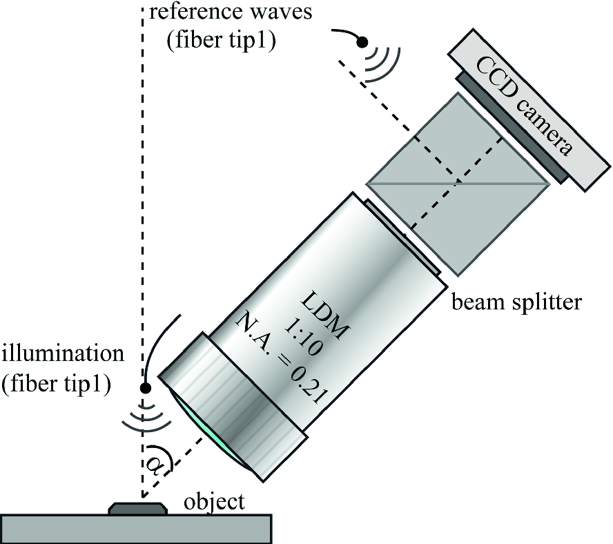
Digital holographic microscope setup (DHM): To image the surface of the test object onto the utilized camera sensor, a long-distance microscope objective (LDM) with a 10× magnification, a numerical aperture N.A. = 0.21 and a working distance of 51 mm is employed. Optical fibers serve to illuminate the object under test and provide a spherical reference wave. For simplicity, only one illumination and one reference is shown. A beam splitter combines the object and the reference waves, producing a hologram across the camera plane
In the following, the 3D surface measurements of the micro cup based on digital holographic microscopy will be discussed; this is the backbone of geometric inspection.
 nm and the other two with
  nm. According to Eq. 5.2, a synthetic wavelength of 69.07 µm results for the evaluation. Utilizing a fiber switch and a 1 × 2 fiber splitter, object and reference waves are formed. A digital hologram captured using the DHM is utilized for recovering the phase and the real amplitude of a monochromatic wave field across the object plane. The hologram generated across the output plane of the DHM is given by
Digital holographic microscopy (DHM) setup based on the scheme of the individual DHM shown in Fig. 5.1. The setup consists of four DHM units distributed around the test object shown in the coherence tomography image in the inset with a diameter of approximately 1 mm and a depth of 0.5 mm. Each unit delivers a measurement of a part of the test object. These four parts are then used to reconstruct the whole 3D shape of the test object. The long-distance microscope (LDM) is an object side telecentric objective with a numerical aperture of 0.21, a magnification of 10× and a working distance of 51 mm. The camera sensor has 2750 × 2200 pixels with a pixel pitch of 4.54 µm


![$$ {\text{I}}({\text{X}}) = \left| {{\text{H}}_{{\uplambda{\text{n}}}} ({\text{X}})} \right|^{2} = {\text{A}}({\text{X}}) + \sum\limits_{{{\text{n}} = 1}}^{\text{N}} {\left[ {\left( {{\text{U}}_{{{\text{O}}_{{\uplambda{\text{n}}}} }}^{*} \cdot {\text{U}}_{{{\text{R}}_{{\uplambda{\text{n}}}} }} } \right)({\text{X}}) + \left( {{\text{U}}_{{{\text{O}}_{{\uplambda{\text{n}}}} }} \cdot {\text{U}}_{{{\text{R}}_{{\uplambda{\text{n}}}} }}^{*} } \right)({\text{X}})} \right]} . $$](../images/463048_1_En_5_Chapter/463048_1_En_5_Chapter_TeX_Equ5.png)

 ) on Eq. 5.5 results in
![$$ \begin{aligned} {\hat{\text{I}}}(\upupsilon) & = {\hat{\text{A}}}(\upupsilon) + \sum\limits_{{{\text{n}} = 1}}^{\text{N}} {\left[ {{\Im }\left\{ {\left( {{\text{U}}_{{{\text{O}}_{{\uplambda{\text{n}}}} }}^{*} \cdot {\text{U}}_{{{\text{R}}_{{\uplambda{\text{n}}}} }} } \right)} \right\}(\upupsilon) \otimes\updelta\left( {\upupsilon +\upupsilon_{{0,\uplambda_{\text{n}} }} } \right)} \right.} \\ & \quad + \left. {\Im \left\{ {\left( {{\text{U}}_{{{\text{O}}_{{\uplambda{\text{n}}}} }} \cdot {\text{U}}_{{{\text{R}}_{{\uplambda{\text{n}}}} }}^{*} } \right)} \right\}(\upupsilon) \otimes\updelta\left( {\upupsilon +\upupsilon_{{0,\uplambda_{\text{n}} }} } \right)} \right], \\ \end{aligned} $$](../images/463048_1_En_5_Chapter/463048_1_En_5_Chapter_TeX_Equ7.png)

a shows a single hologram, which contains object information for 4 directions of illumination and b shows the corresponding spectrum with four ± first order and the central dc components
It is noteworthy that the test object is illuminated from four different directions and four holograms are recorded on a single shot using four reference waves by applying the digital holography multiplexing principle [Ago17]. These holograms are used to reduce speckle noise in two-wavelength contouring. Accordingly, each holographic unit from the four units will capture two successive multiplexed holograms. The two successive multiplexed holograms are captured, one for each wavelength. In the following, the results that were obtained using the four observation directions will be presented and discussed. The time required for the capturing process and for the switching between the two wavelengths is 120 ms. Using the spatial carrier frequency method [Ago15], one can numerically reconstruct the phase distributions ϕλ1 and ϕλ2, which correspond to the two measurements.
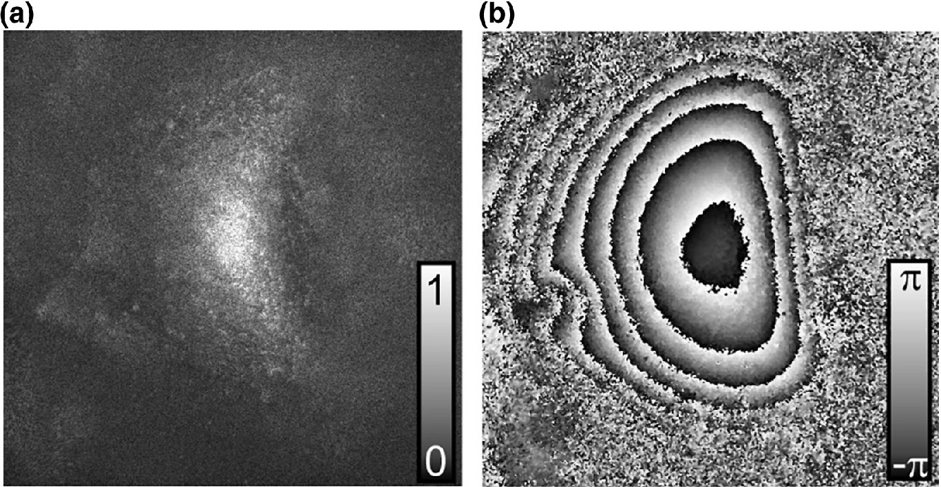
a Image of the real amplitude of the reconstructed complex amplitude across the capturing plane of the recorded hologram for  nm. b Image of the phase difference Δ = ϕλ2−ϕλ1 between the two reconstructed phase distributions across the capturing plane. The image size is 2200 × 2200 pixels with a pixel pitch of 4.54 µm

a Image of the real amplitude, which represents a sharp image of the micro cup under test with respect to the observation direction. b Image of the phase difference distribution, which represents a sharp contouring phase map across the whole object
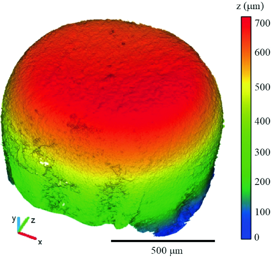
The 3D height map calculated after unwrapping the countering phase maps obtained from the four holographic systems
5.2.3 Dimensional Inspection
Dimensional inspection implies the evaluation of surface data with respect to dimensional, form and position deviations of certain geometric features. These deviations are compared to the specified tolerances in order to decide whether the workpiece meets the quality requirements or not. The following subsections give a brief survey of the state of the art in evaluating point clouds and present the holistic approximation as the method of choice for the dimensional inspection of optically acquired surfaces of micro parts.
5.2.3.1 State of the Art
- 1.
Neighboring measurement points are rated based on their curvature and assigned to corresponding geometric elements [Wes06]. This method can provide accurate solutions, but it is sensitive to noisy data and not able to distinguish between spheres and cylinders with certain radii.
- 2.
A holistic approximation can evaluate a composed set of data under the present boundary conditions in a single approximation task [Goc91]. By the definition of separating functions, an optimal assignment of the measurement points to the corresponding geometric elements (segmentation) can be carried out simultaneously. The method is presented for different applications, e.g. for a 2D combination of lines and circles [Lüb10], or for micro punches as a 3D combination of a cylinder, a torus and a plane [Lüb12].
It was proved that the holistic approximation with automated segmentation (second approach) is only slightly sensitive regarding the initial values of the approximation and at the same time converges reliably within wide ranges [Lüb10]. Furthermore, this method was successfully tested for the evaluation of micro-measurements [Zha11], and it allows the automatic detection of outliers by a combination with statistical methods [Gru69]. Thus, the second approach is particularly suited for noisy optical measurement data. However, the algorithms have not yet been implemented for the evaluation of optical data acquired with DHM.
5.2.3.2 Method
 , while the position of the elements is included in a transformation vector
  . The detailed principle of the holistic approximation is described in [Goc91] for 2D combinations and in [Lüb12] for a 3D application. The approximation is performed by minimizing the L2 norm
Cross-section of micro cup model composed from geometric primitives (cylinder, torus, and plane) in the workpiece coordinate system (WCS) with segmentation elements according to the geometric model
![$$ \begin{array}{*{20}c} {\mathop {\hbox{min} }\limits_{{\overrightarrow {\varvec{a}}_{p} , \overrightarrow {\varvec{a}}_{g} }} \left[ {\mathop \sum \limits_{i = 1}^{{n_{cyl} }} \left( {d_{i,cyl} \left( {\overrightarrow {\varvec{a}}_{p} , \overrightarrow {\varvec{a}}_{g} } \right)} \right)^{2} + \mathop \sum \limits_{i = 1}^{{n_{tor} }} \left( {d_{i,tor} \left( {\overrightarrow {\varvec{a}}_{p} ,\overrightarrow {\varvec{a}}_{g} } \right)} \right)^{2} } \right.} \\ {\left. { + \mathop \sum \limits_{i = 1}^{{n_{pla} }} \left( {d_{i,pla} \left( {\overrightarrow {\varvec{a}}_{p} ,\overrightarrow {\varvec{a}}_{g} } \right)} \right)^{2} } \right]^{1/2} ,} \\ \end{array} $$](../images/463048_1_En_5_Chapter/463048_1_En_5_Chapter_TeX_Equ8.png)
 and shape parameters
  ) are optimized, but also the assignment of the measurement points to the geometric elements. This implies that the numbers of elements in Eq. 5.7 vary during the iterative calculation. The geometric assignment itself is based on a geometric model, which is presented as a cross-section in Fig. 5.7. It consists of a cylinder with radius rc, whose axis represents the z-axis, a quarter of a torus in the x–y-plane with wall radius rw and ring radius rr = rc − rw as well as a plane parallel to the x–y-plane at z = −rw. This model contains certain geometric constraints, e.g. coaxiality of the cylinder and the torus axis, which are again perpendicular to the plane, as well as tangential transitions between all elements. These constraints result from the workpiece design and reduce the degrees of freedom to five transformation parameters
 ![$$ \overrightarrow {\varvec{a}}_{p} = \left[ {\Delta x,\Delta y,\Delta z,\varphi_{x} ,\varphi_{y} } \right] $$](../images/463048_1_En_5_Chapter/463048_1_En_5_Chapter_TeX_IEq9.png) and two shape parameters
and two shape parameters ![$$ \overrightarrow {\varvec{a}}_{g} = \left[ {r_{c} ,r_{w} } \right] $$](../images/463048_1_En_5_Chapter/463048_1_En_5_Chapter_TeX_IEq10.png) . As the geometry is axially symmetric, the rotation
. As the geometry is axially symmetric, the rotation  around the z-axis remains disregarded.
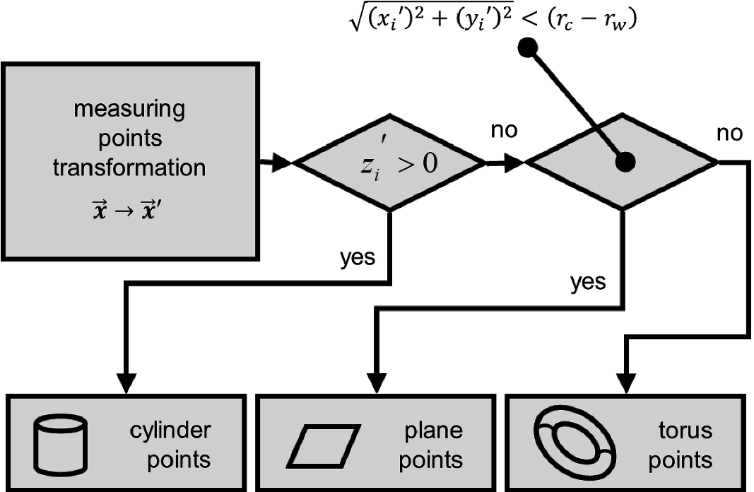
Decision rules for assigning the measured points to the geometric primitives. All points with a positive z-coordinate are assigned to the cylinder; the remaining points are distinguished by their polar radius. Points with a radius ri < (rc − rw) belong to the plane, the residual points are assigned to the torus
5.2.3.3 Verification and Measurement Results

Approximation results for simulated data (ca. 800,000 points) with different intervals of noise ae: mean values of the radius deviations for cylinder  and torus
  with standard deviations
 and
and  are introduced and the coverage factors
 and
and  , respectively, based on the mean approximated radii
  ,
,  of the cylinder and the torus as well as their standard deviations σc, σw.
The maximum value for the cylinder radius is tc,max = 0.74, whereas it is tw,max = 0.92 for the torus radius. According to the t-distribution for a probability of 95% (α = 0.05) and a degree of freedom of f = n−1 = 99, the critical value is tcrit = 1.984. As both calculated coverage factors are below this critical value, it can be stated that the verification results do not disagree with the hypothesis with a probability of error of 5%. Thus, it can be assumed that no systematic influence within the holistic approximation leads to significant deviations of both the approximated radii.
The random deviations can be characterized by the standard deviations of the calculated radii. In absolute numbers, the standard deviation of the cylinder radius is σc < 22 nm in this simulation, while the standard deviation of the torus radius is σw < 2.87 µm. The random deviations of the torus are 2 orders of magnitude higher than those of the cylinder radius, which is assumed to result from the approximation of only a part of the geometric torus object and agrees with earlier findings, e.g., the error of a spherical center approximation depending on the size of the measured spherical cap [Bou93], or the increased diameter [Fla01] or center uncertainty [McC79] with decreasing arcs of a circle. A second reason for the increased standard deviation of the torus radius might be the number of evaluated points. The torus was simulated with approximately 100,000 points, which is only a third of the number of points on the cylinder. Nevertheless, for both parameters the standard deviation is only a fraction of the initial amplitude of noise due to the high number of data points available.
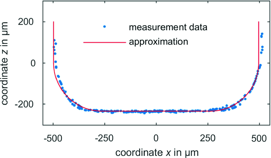
Cross-section of the acquired data (measurement data, see Fig. 5.6) with the result of the holistic approximation. Note that shape deviations of the cylindrical part of the three-dimensional micro cup are responsible for the systematic deviations between the measured and approximated data points in the cross-section shown
5.2.4 Detection of Surface Defects
Surface defects such as scratches or dirt might be too small to cause a detectable change in the measured phase distribution. Hence, reliable detection necessitates additional methods, which incorporate the measured amplitude image.
5.2.4.1 State of the Art
Currently, algorithms for automatic surface inspection are to a large extent based on manually engineered features [Xie08], most commonly statistical and filter-based [Neo14]. While the introduction of expert knowledge often allows for the creation of powerful features, this process is laborious and might be necessary for each new product. General solutions that can automatically adapt to new problem sets could thus yield significant time and cost advantages. One such solution is convolutional neural networks (CNN). These have become the driving factor behind many recent innovations in the field of computer vision and allowed significant advances in various applications, such as object classification [Kri12] or semantic image segmentation [Yu15]. CNNs have also recently been successfully applied for industrial surface inspection [Wei16].
5.2.4.2 Methods
The core building block of CNNs is the convolutional layer. Instead of processing, e.g. an image all at once, it is divided into small (usually) overlapping windows and fed piece-wise into a neural network. Each window is thus mapped to a vector of activations of a shared neural network. Convolutional layers hence automatically learn a set of filters in the form of the networks weights.
In the most common framework, convolutional layers are combined with pooling layers, usually max-pooling layers. Max-pooling layers summarize the extracted features by taking the maximum activation for each unit over a small area. Deep CNNs are built by stringing together multiple convolutional and pooling layers. With increasing depth, the network thus extracts increasingly complex features for increasingly large image areas or receptive fields. The application of max-pooling thereby yields multiple advantages. By scaling down the input, the number of parameters is decreased, which increases the computational efficiency. At the same time, the receptive field sizes are increased and hence the amount of context that can be integrated by each unit of the neural network. Additionally, the use of max-pooling yields a small degree of translation invariance, which increases the network’s robustness towards these operations. One disadvantage, however, is that, by scaling down the input, spatial resolution gets lost. This becomes an issue when the goal is spatially precise defect detection. To solve this problem, multiple solutions have been proposed in the field of semantic image segmentation, e.g. the use of dilated convolutions [Yu15], the U-Net architecture [Ron15] and the LinkNet architecture [Cha17].
One solution is to augment the classical CNN architecture with a second network for upscaling the spatial resolution. High-level, low-resolution features are thereby up-sampled and merged with the corresponding low-level, high-resolution features. This architecture is largely known as U-Net [Ron15]. The advantage is that it harnesses the benefits of max-pooling while still being able to give precise defect labels.
Here we implemented a modified version of the U-Net. Aside from accurate defect detection, our objective was thereby to keep the hardware requirements and computing time of the network as low as possible. To achieve this goal, we employed three recently developed methods. Firstly, our architecture is heavily inspired by densely connected CNNs [Hua17]. Secondly, we opted for depth-wise separable convolutions [Cho16]. Finally, our network takes inspiration from the LinkNet architecture [Cha17].
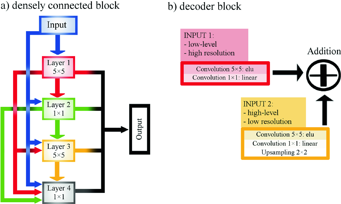
a Densely connected block as used in this work. The Input (blue) is fed into all successive layers of the block. The activations of each layer (red, green, orange, gray) are fed into all successive layers. The output is constructed by concatenating the activations of all layers of the block (red, green, orange, gray), but not the input. b Decoder block to integrate low- and high-level features. Input 1 (upper left): Low-level features are subjected to one non-linear (exponential linear unit: elu) and one linear 1 × 1 convolution. The number of features is thereby reduced by a factor of 0.25. Input 2 (lower right): High-level features are subjected to one non-linear and one linear 1 × 1 convolution and then sampled up to match the resolution of the low-level input. The number of features is thereby also reduced to match the reduced low-level features
Layer types, filter sizes, number of units and input/output dimensions for each layer within a block (W: width, H: height, SC: separable convolution)
Layer type | Filter size | # units | Input resolution | Output resolution |
|---|---|---|---|---|
Input | d | – | W × H × d | |
SC | 5×5 | h | W × H × d | W × H × h |
SC | 1×1 | h | W × H × h+d | W × H × h |
SC | 5×5 | h | W× H × 2∙h+d | W × H × h |
SC | 1×1 | h | W × H × 3∙h+d | W × H × h |
Output | – | W × H × 4∙h |
The second method for increasing the model efficiency is the use of depth-wise separable convolutions [Cho16]. The principle behind depth-wise separable convolutions is that, instead of performing convolutions over all channels within a spatial window simultaneously, the spatial and the depth/channel-wise convolutions are performed separately. This allows for a significant decrease in the amount of network connections.
The third method for increasing the model efficiency takes inspiration from the LinkNet architecture [Cha17]. There are two ways in which LinkNet increases the efficiency of the standard U-Net architecture. Firstly, high- and low-level features are merged via addition instead of concatenation. Secondly, the number of features is also reduced before the summation. Our implementation of this procedure is shown in Fig. 5.11b.
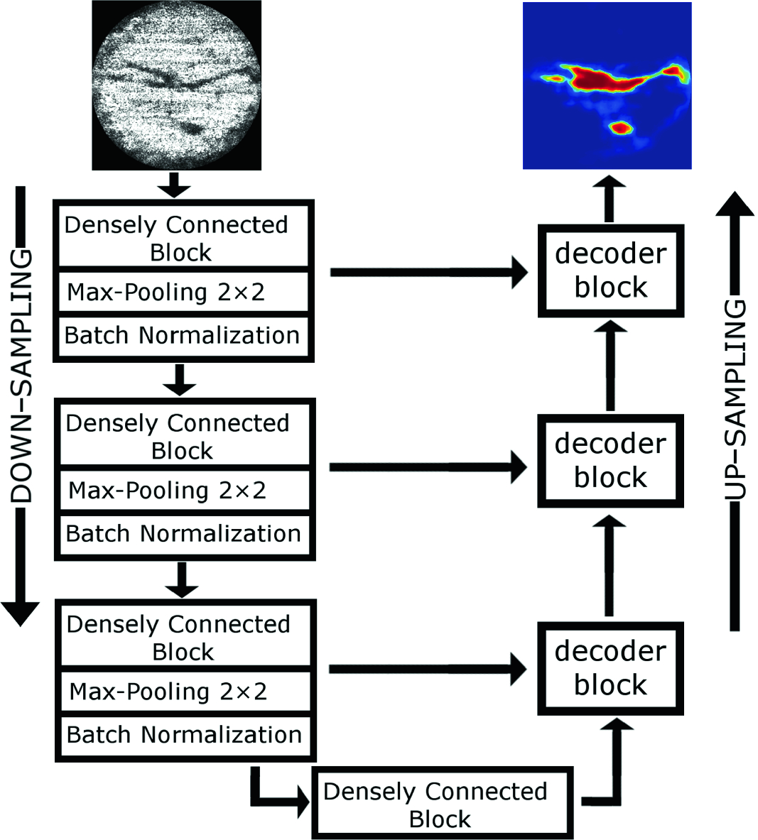
Dense U-Net as implemented for this work. The picture on the upper left shows the input image of the test part to be inspected, while the result on the upper right shows the predicted defect position. In the down-sampling part, the input is fed into blocks of densely connected convolutional layers (see Fig. 5.11a), followed by 4 × 4 max-pooling and batch normalization. The up-sampling part uses decoder blocks as described in Fig. 5.11b. The spatial resolution is restored via up-sampling and concatenation with the corresponding layer of the down-sampling part as well as another densely connected block
As activation functions, we used exponential linear units (elu) [Cle15] in all but the output layers. For the output layer, we used sigmoid units to constrain the output to the interval [0, 1]. The network was trained by minimizing binary cross-entropy (also known as log-loss) using the Adam optimizer [Kin14]. The learning rate was initialized at 0.001 and automatically reduced by a factor of 0.1 when no decrease in loss was observed for more than 10 epochs. The mini-batch size was set to eight. All experiments were conducted using the keras library for Python.
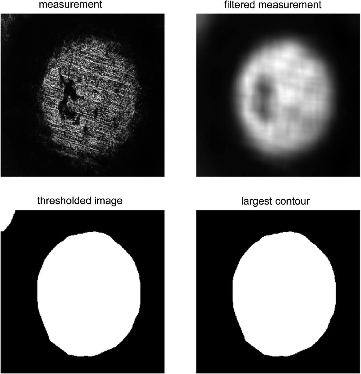
Background removal: In order to improve defect detection, the background was removed from the final classification result. The measurement (upper left) was low-pass filtered. The resulting image (upper right) was thresholded by its mean value. In the resulting image (lower left) the largest contour was detected and used as a mask for background removal (lower right)
We evaluated our method by using 64 samples for training and the remaining 5 samples for evaluation. To increase the amount of training data artificially, we used the following operations: horizontal flipping, vertical flipping, random rotations, and scaling the size by a factor between 0.9 and 1.1 (cropping or adding the additional/missing pixels at the boundaries).
5.2.4.3 Validation
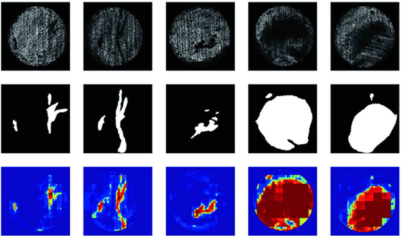
Network prediction for all five test measurements. Top row: input measurement after background subtraction. Middle row: defect masks. Bottom row: defect predictions. All defects are marked correctly
Defect detection for a single input image takes <130 ms on our test system (AMD Ryzen Threadripper 1900X 8-Core Processor × 16, 64 GB RAM, GeForce GTX 1080 Ti). Additional speed gains can be achieved by processing multiple images at once, as this would decrease the amount of data transfer towards and from the Graphics Processing Unit (GPU).
Acknowledgements The editors and authors of this book like to thank the Deutsche Forschungsgemeinschaft DFG (German Research Foundation) for the financial support of the SFB 747 “Mikrokaltumformen—Prozesse, Charakerisierung, Optimierung” (Collaborative Research Center “Micro Cold Forming—Processes, Characterization, Optimization”). We also like to thank our members and project partners of the industrial working group as well as our international research partners for their successful cooperation.
5.3 Inspection of Functional Surfaces on Micro Components in the Interior of Cavities
Aleksandar Simic*, Benjamin Staar, Claas Falldorf, Michael Lütjen, Michael Freitag and Ralf B. Bergmann
Abstract A fast and precise solution for the inspection of the interior of micro parts using digital holography is presented in this chapter. The system presented here is capable of operating in an industrial environment. For this purpose, a compact Michelson setup in front of the imaging optics is used, so that the light paths of the object- and reference arm are almost identical. This makes the system less vulnerable to mechanical vibrations. A further improvement is obtained using the two-frame phase-shifting method for the recording of a complex wave field. This enables the usage of two cameras in order to allow the recording of a complex wave field in a single exposure. With the help of two-wavelength contouring, optically rough objects with a synthetic wavelength of approximately 93 µm are investigated. The measurement results make it possible to determine the shape of the interior surface and faults such as scratches with a resolution of approximately 5 µm. In order to fully utilize the measurement speed of the setup, a fast and reliable solution for automatic defect detection is required. For a profitable industrial application, it is therefore crucial to reliably detect all defective parts while producing little to no false positives (i.e. pseudo-rejections). This is realized by utilizing prior knowledge about the object shapes to implement fast phase unwrapping for defect detection. Defects are then reliably detected by identifying consecutive areas of deviation in relative depth. The evaluation of measurements taken in an industrial environment shows that this approach reliably detects all defects with a false-positive rate of less than one percent.
Keywords Quality control · Optical monitoring · Digital holography
5.3.1 Introduction
Micro cold formed parts are produced in high quantities, as many of such are incorporated inside a complete system. The mass production of micro parts can only be efficient if the quality inspection of these parts is incorporated within the production line. Optical metrology offers the opportunity to determine the shape of the structures of such parts and allows for quality control. Automated quality control with the help of an automated optical system within the industrial production line reduces the costs and time that would otherwise be required for a sophisticated manual inspection. Up to now, tactile methods have been used to inspect components on a sample basis, but these are not suitable for fast quality inspection in the production line as they are too slow and might alter the sample.
Among the non-tactile methods, confocal microscopy is commonly used for inspection but is clearly too slow for an automated 100% inspection. An overview of such methods can be found in [Ber12, Kop13]. Alternatively, white-light interferometry (WLI) is suitable, as it measures with high speed and is highly precise. For a review of WLI, see [Gro15]. However, WLI requires a comparatively large number of recordings, commonly by depth scanning, to capture depth information.
Digital holography (DH) is precise and only requires a small number of recordings to obtain the object shape, as shown in [Fal15]. This makes it a good candidate for the fast three-dimensional inspection of micro parts. Usually DH uses the method of temporal phase-shifting for phase evaluation, which is generally realized with a piezoelectric device. To realize a system which exhibits an even higher robustness, the method of two-frame phase-shifting is used to measure the object shape in two consecutive exposures.
5.3.1.1 Digital Holography
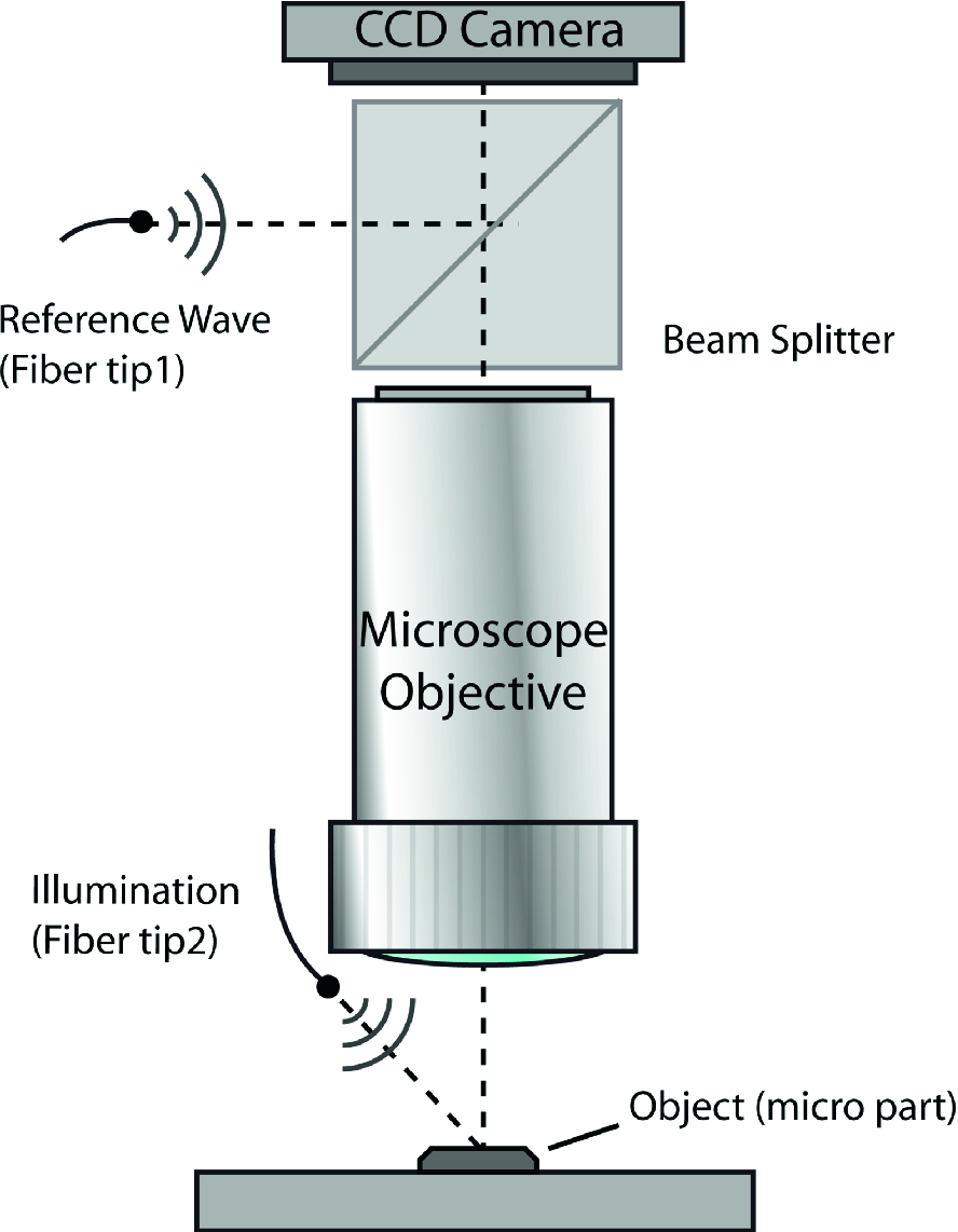
Sketch of a conventional setup in digital holography. The object (micro part) is illuminated and the image is magnified with the help of a microscope objective and projected on a CCD camera. At the same time, the CCD is illuminated with a reference wave. The arising interference pattern gives the opportunity to extract the complex wave field [Ago17]

 is the position vector and
  and
and  are the object- and reference-wave fields respectively, with
  and
and  being the particular conjugated wave fields. When multiplying this interference pattern with the complex amplitude of the reference wave, the following fundamental equation is obtained:
 of the object. The last term represents a virtual image of the object. The phase Φ of the wave field
  contains information on the form of the object. The height h of the observed object can be calculated with the phase Φ from
5.3.1.2 Two-Wavelength Contouring
 and
and  . The corresponding phase distributions are subtracted and the resulting phase difference can be interpreted as a single measurement with a synthetic wavelength [Fal15] of
The synthetic wavelength can be chosen to be much larger than the surface roughness by adjusting  and
and  to resolve the ambiguity problem.
5.3.1.3 Two-Frame Phase-Shifting
The recorded digital hologram from Eq. 5.11 only contains object information in the virtual image, and the remaining inverted image and DC term are generally not of interest. Therefore, only a small part of the camera resolution can be used with this method. To use the complete spatial bandwidth, the method of temporal phase-shifting is used, where the phase is shifted by a fractional amount of the wavelength to generate several equations and extract detailed phase information.
 of the involved wave fields, to extract 3D-information on the considered object by using
This equation contains the three unknown variables  which makes it impossible to extract the phase difference
  . To solve this problem the phase difference
  of the interference pattern produced is shifted with a known factor
  to obtain a system of at least three equations from the corresponding recorded intensities. This process is generally accomplished with the help of a piezoelectric device in the setup. The resulting phase distribution is wrapped in the bounded interval [0, 2π] and has to be unwrapped to determine the continuous behavior.
To incorporate this method in an industrial environment, its robustness is improved by replacing the piezoelectric device. To maintain the complete space–bandwidth product of the detected signal, it is vital to find a way of using temporal phase-shifting in a single camera exposure. For this purpose, the temporal phase-shifting method is used with the help of only two recorded interference patterns. This is accomplished by using circular polarized light from the object and linear polarized light from the reference mirror. Nozawa et al. have already used this system for single-shot and highly accurate measurements of complex amplitude fields with a simple optical setup [Noz15].
 in the CCD plane can be written as
 and
and  being the phase-shifted single recorded interference patterns shifted by
  , respectively. Liu et al. showed that the DC term
  is given by [Liu09]
5.3.2 Experimental Alignment
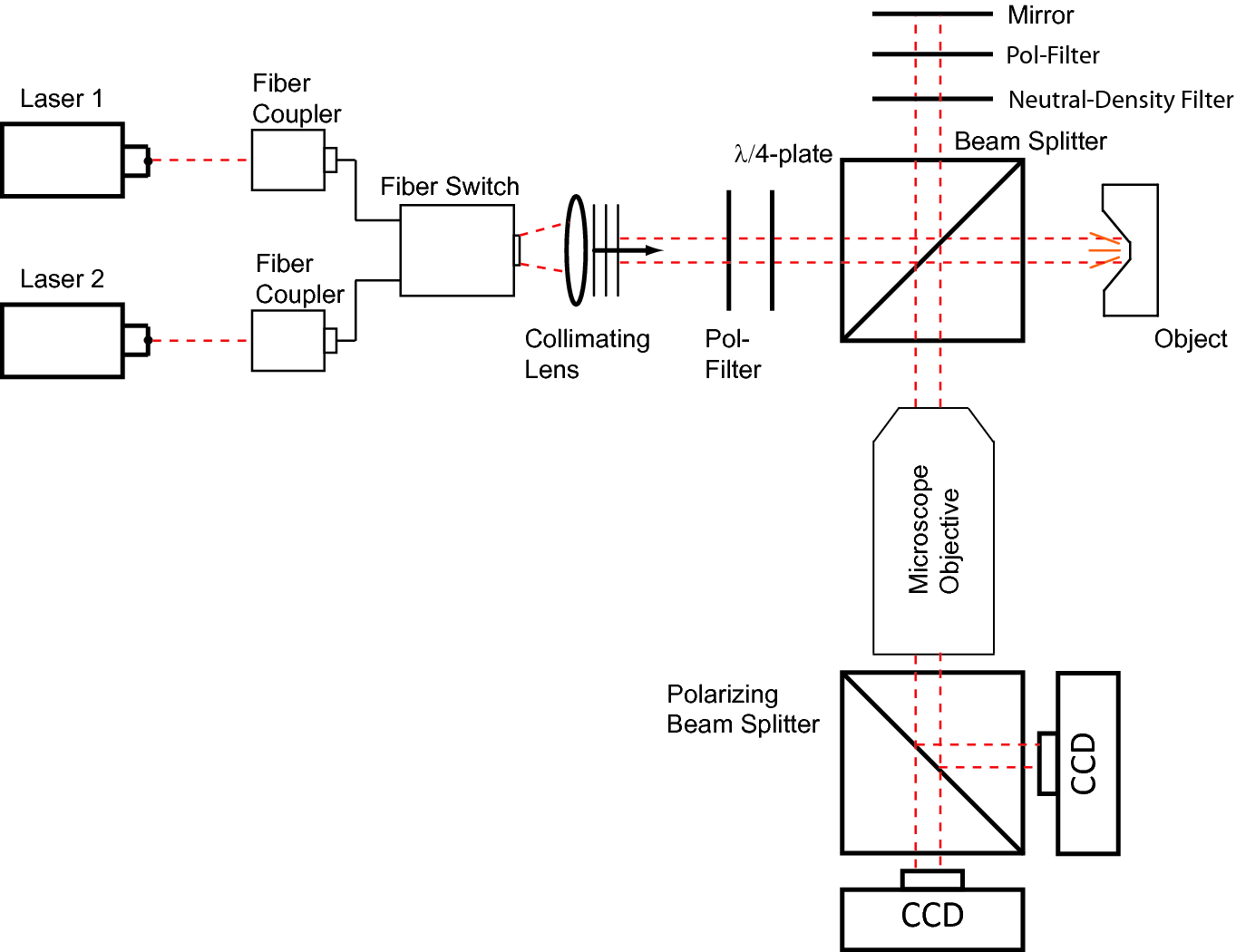
Setup for the internal inspection of micro deep-drawing parts. Before entering the interferometer shown in the right part of the drawing, the light is polarized circularly with a λ/4-plate. The interferometer consists of a mirror in one arm and an object in the other arm. With the help of a polarizing filter, the reference light is polarized linearly while the object wave has a circular polarization. The image is magnified 5x using the microscope objective. By using a polarizing beam splitter, two interference patterns are projected on two cameras at the same time, being shifted by 90°
After leaving the fiber switch, the light is parallelized with the help of a collimating lens and is linearly polarized. A λ/4 plate then polarizes the light circularly and illuminates the object through a beam splitter. At the same time, half of the intensity is redirected and linearly polarized again to illuminate the reference mirror. After traveling through a microscope with 5x magnification, the light is again divided with the help of a polarization-sensitive beam splitter to lead it to two camera targets at the same time. By using such a beam splitter, two interference patterns are projected on the camera targets, shifted by 90°.
As light sources, two diode lasers with output powers of  mW and
  mW and with wavelengths
  nm and
  nm are used. With that, the camera exposure times were set to 8 ms to fully illuminate the camera targets. With the employed wavelengths, the synthetic wavelength amounts to
  µm. To avoid coherent amplification and to minimize speckle noise, laser light with coherence lengths of less than 1 mm is used.
5.3.2.1 Experimental Results
Sketch of the investigated micro part. The area marked in light red around the lower hole serves as a functional area and has to be inspected.
Taken from [Sim17]
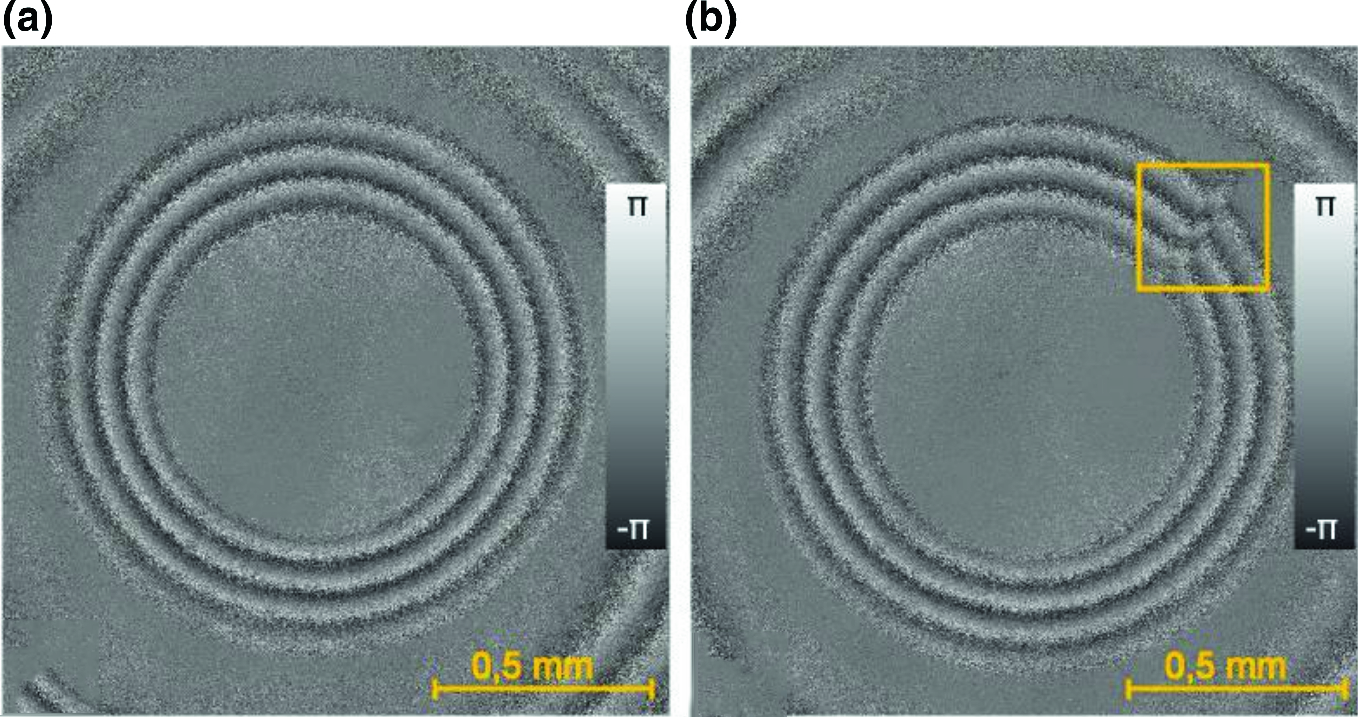
a Phase distribution of the recorded functional area of the inspected micro part, which is an acceptable part. In b one can see the function area with a potential fault.
Taken from [Sim17]
 at the dotted lines of
Defect detected in the functional area after unwrapping the detected phase. The mean depth of the scratch is calculated on the dotted lines and amounts to d(x, y) = (20.2 ± 1.5) µm.
Taken from [Sim17]

With this system, a lateral as well as a depth resolution of 5 µm can be achieved.
5.3.2.2 Comparison with X-Ray Tomography

a Measured spot on the functional surface with X-ray tomography. b Cross-section with the result of the depth measurement
5.3.2.3 Different Batches of Material
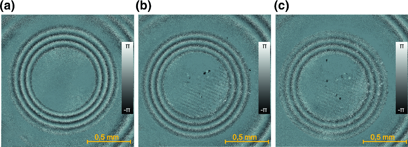
Measurements of the same part of different batches of a heat-treated, b oily and c glossy material. The signal-to-noise ratio decreases for oily and glossy parts and does not allow a precise evaluation
5.3.3 Automatic Defect Detection
For the effective utilization of the setup’s measurement speed, manual evaluation of the measurements is not feasible. Hence a solution for automatic defect detection was developed. Thus the challenge was threefold: Firstly, the method had to be fast, as a slow algorithm would be detrimental to the fast measurement system. Secondly, defect detection had to be very accurate, with zero false negatives (undetected defects) and less than 4% false positives (intact parts falsely labeled as defective). Thirdly, due to the well optimized process, the number of defective samples was very small. Consequently, the application of state-of-the-art machine learning methods, like e.g. convolutional neural networks, which have been applied by Ronneberger et al. [Ron15] and Weimar et al. [Wei16] for example, was not feasible.
 . Potential defects are then filtered out by applying a low-pass filter (LPF) in a circular motion. The resulting prototype is then subtracted from the measured
  to identify deviations via the application of a threshold. The whole defect detection pipeline is schematically shown in Fig. 5.22.
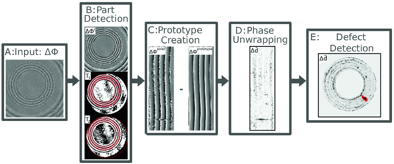
Defect detection pipeline. a: phase distribution image ΔΦ. b: Circles are detected in the phase distribution image ΔΦ via thresholding and contour detection. c: A defect-free prototype,  , is created by mapping ΔΦ to polar coordinates, yielding
  and applying a LPF in the angular direction. d: Phase unwrapping is realized by subtracting the prototype
  from
from  , yielding the depth deviation image
  . e: Defects are identified from
  and marked accordingly (mapped back to Cartesian coordinates for better visualization)
5.3.3.1 Preprocessing
In order to decrease noise,  was filtered by applying a sin/cos LPF. Since
  is a phase distribution, low-pass filtering in the complex plane may be applied, i.e. to the complex phasor
  which exhibits unit amplitude and
  as the phase. This approach prevents filter artifacts at the phase transitions.
5.3.3.2 Part Detection
 , yielding
  and subsequently applying a binary threshold to
  resulting in two images
  and
and  with:
with:
An example is shown in Fig. 5.22b. Subsequently, contours in  and
and  are detected and sorted by area. The largest contours are then fitted by their minimal enclosing circle. As a robust estimate of the object’s center, the median of the resulting centers is taken, yielding the center
  .
.
5.3.3.3 Prototype Creation and Phase Unwrapping
In order to detect defects, the measured phase distribution  is compared to an ideal prototype of that measurement. Expecting the measured part to have a smooth surface, prototype creation is achieved by the application of a sin/cos low-pass filter in a circular motion. One could think of this as virtually regrinding the object to smooth out defects. The detailed steps for this process are as follows:
 is mapped to polar coordinates with respect to the object’s center detected in the previous step. The result is an
  image
image  whereby
  marks the angular resolution and r the radius.
![$$ \begin{array}{*{20}c} {\Delta\Phi ^{\text{polar}} \left[ {{\text{x}},{\text{y}}} \right] = \Delta\Phi \left[ {{\text{y}} \cdot { \cos }\left( {\frac{{{\text{x}}2\uppi}}{\upbeta}} \right) + {\text{c}}_{\text{x}} ,{\text{y}} \cdot { \sin }\left( {\frac{{{\text{x}}2\uppi}}{\upbeta}} \right) + {\text{c}}_{\text{y}} } \right]} \\ {{\text{x}} = 1, \ldots ,\upbeta \in {\mathbb{N}}} \\ {{\text{y}} = 1, \ldots ,{\text{r }} \in {\mathbb{N}}} \\ \end{array} $$](../images/463048_1_En_5_Chapter/463048_1_En_5_Chapter_TeX_Equ19.png)
 , yielding
  (for an example see Fig. 5.22c). The
  filter matrix was thereby chosen to be much larger in angular direction m than in radial direction n. The reasoning is that, due to phase transitions, high-frequency components are expected in the radial direction even for smooth surfaces. In the angular direction, however, a smooth surface should only exhibit low-frequency components, as there should not be any phase transitions. Deviations in depth can thus be calculated via (Fig. 5.22d)
5.3.3.4 Defect Detection
Potential defects are marked by deviations from zero in  . Due to roughness of the measured part’s surface that lies within tolerance, there might exist multiple such areas, even for intact parts. To differentiate between this background noise and actual defects, two different features are used. Firstly, errors are assumed to be marked by larger connected areas of deviations from zero, i.e., the area of an actual defect exceeds a certain threshold. Secondly, it is assumed that for defective areas the mean deviation from the background exceeds a certain threshold.
Accordingly, the defect detection routine searches for connected areas of deviations from zero in  with areas above an area threshold
  where the mean deviation exceeds a depth threshold
  . An example is shown in Fig. 5.22e.
5.3.3.5 Detecting Loss of Focus
 is employed. The underlying assumption is that well focused parts of
  show homogeneous orientation of gradients, while unfocused areas show gradient orientations that are more or less random. Focused areas are hence marked by low standard deviation in the gradient orientations, while unfocused areas are marked by large standard deviation. The gradient orientation in
  is calculated in the following way. First, the Sobel derivatives [Sob90] are calculated by convolution with Sobel operators
  and
and  , resulting in
![$$ {\text{G}}_{\text{x}} = {\text{S}}_{\text{x}} *\Delta\Phi ^{\text{polar}} = \left[ {\begin{array}{*{20}c} 1 & 0 & { - 1} \\ 2 & 0 & { - 2} \\ 1 & 0 & { - 1} \\ \end{array} } \right] * \Delta\Phi ^{\text{polar}} $$](../images/463048_1_En_5_Chapter/463048_1_En_5_Chapter_TeX_Equ21.png)
![$$ {\text{G}}_{\text{y}} = {\text{S}}_{\text{y}} *\Delta\Phi ^{\text{polar}} = \left[ {\begin{array}{*{20}c} 1 & 2 & 1 \\ 0 & 0 & 0 \\ { - 1} & { - 2} & { - 1} \\ \end{array} } \right] *\Delta\Phi ^{\text{polar}} . $$](../images/463048_1_En_5_Chapter/463048_1_En_5_Chapter_TeX_Equ22.png)
 and
and  with absolute values above five times the median absolute deviation (mad), i.e.
  and
and  respectively. The identified values are then replaced by the respective median value (Fig. 5.23c).
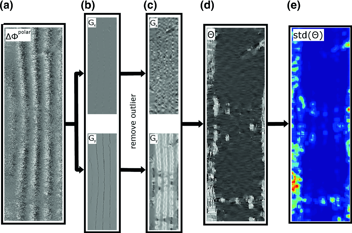
a: Polar coordinate image  of the phase distribution
  . b: Result of calculating Sobel derivative of
  in x- and y-direction (
 and
and  respectively). c: Result of removing outlier derivatives caused by phase transitions. d: The gradient orientation image
  . e: Local standard deviation of gradient orientation image
  . Blue marks low values while red marks large values

 of
of  over windows of
  pixels is calculated
 unit matrix
  as the convolution kernel. The normalized sum f of the values in
  then serves as an indicator value on how focused the image is (Fig. 5.23e):
If  exceeds a certain threshold
  , the measurement is said to be out of focus.
5.3.3.6 Results
 , depth
  and focus
  . After evaluating different settings manually, the set of parameters shown in Table 5.2 was used for further work
Parameter set for defect routine
Parameter | Variable | Value |
|---|---|---|
Angular resolution |
| 1800 pixels |
Threshold: area |
| 1000 pixels |
Threshold: mean depth |
| 0.1 (Range: 0–2 |
Threshold: focus |
| 0.07 |


Defect detection was evaluated on 296 measurements of 247 parts (230 parts of those were previously inspected and found to be acceptable and 17 parts were identified as bad parts) in the department of quality assurance of Stüken Corp. with a measurement speed of approximately one part per second. Defective parts were all measured at least 3 times with different orientations to verify reproducible defect detection. Out of the 296 measurements, all the defective parts were reliably detected (true positive), while eleven intact parts were sorted out. Of these eleven parts, nine were correctly sorted out due to the measurement being out of focus, leaving two false positive detections.
Acknowledgements The editors and authors of this book like to thank the Deutsche Forschungsgemeinschaft DFG (German Research Foundation) for the financial support of the SFB 747 “Mikrokaltumformen—Prozesse, Charakerisierung, Optimierung” (Collaborative Research Center “Micro Cold Forming—Processes, Characterization, Optimization”). We also like to thank our members and project partners of the industrial working group as well as our international research partners for their successful cooperation.
5.4 In Situ Geometry Measurement Using Confocal Fluorescence Microscopy
Merlin Mikulewitsch* and Andreas Fischer
Abstract Due to the challenging environment of micro manufacturing processes such as laser chemical machining (LCM) where the workpiece is submerged in a fluid, a contactless in situ capable measurement is required for quality control. However, the in situ geometry measurement has several challenges for optical measurement systems because the high surface gradients of the micro geometries and the fluid environment complicate the use of conventional metrology. Confocal fluorescence microscopy allows for the determination of the surface position by adding an isotropically scattering fluorophore to the fluid and detecting the signal drop at the boundary layer between the measured object and the fluid. This technique, capable of improving the measurability of metallic surfaces with strong curvatures, is evaluated for suitability as an in situ measurement method for the LCM process. Unlike in thinner layers, however, the signal with fluid layers ≥1 mm, as needed for LCM in situ applications, shows strong dependencies on the fluorophore concentration and fluid depth. Thus, a physical model of the fluorescence intensity signal was developed for the evaluation of the surface position. To validate the method for the in situ measurement of geometry parameters, the step height of a submerged reference step was determined by measuring the surface positions along a line over the step. The step height measurement results in an uncertainty of 8.8 μm that is verified by deriving the potential measurement uncertainty of the model-based measurement approach. Further investigation of the uncertainty budget will allow a reduction of the measurement uncertainty and enable in situ monitoring and control of the LCM process.
Keywords In situ measurement · Confocal microscopy · Signal modeling
5.4.1 Challenges of Optical Metrology for In-Process and in situ Measurements
Laser chemical machining (LCM) is a promising alternative process that allows for inexpensive manufacturing of micro geometries in hard metals, such as dies for micro forming, without heat damage or structural alterations to the material [Mik17]. Laser chemically machined geometries can reach structure sizes between  and
and  , with steep slopes and a surface roughness of up to
  [Ste10]. However, factors in the process environment, such as chaotic thermal interactions between the fluid and workpiece geometry, complicate the manufacture of a desired geometry, necessitating a closed-loop quality control [Zha17] with an in situ measurement feedback to improve the manufacturing quality (see Sect. 4.3). The challenging conditions of the LCM process, such as the requirement that the workpiece needs to be submerged by a fluid layer (typically 1‒40 mm thick), hinder the in situ application of many measurement methods. The general lack of accessibility to the workpiece, for instance, requires the use of contactless measurement methods based on optical acquisition.
Conventional micro-topography measurement techniques can be separated into interferometric methods (e.g. displacement interferometry, digital holography [Kop13]) and other techniques, such as conventional laser-scanning confocal microscopy [Han06]. Conventional confocal microscopy is hindered, however, by the in situ conditions of high surface angles of the specimen [Liu16]. Interferometric methods were also investigated as a means of control feedback [Zha13], but were found to be unsuitable: The tested measurement systems integrated the interferometer directly into the machining head of the laser jet system as a two-beam interferometer according to the Michelson principle in order to increase the signal strength. The measuring beam was guided coaxially to the etchant and processing beam onto the surface of the workpiece. To obtain the path difference from the interferogram, the number of interference fringes was determined with phototransistors. If the measuring and reference arms are in different ambient media, a correction with the refractive indices of the media is also required. Evaluating the interferometer with samples of different surface roughness, it was determined that the measuring signal strength decreases with increasing surface roughness [Ger10]. In the end however, successful in situ measurement application proved to be unfeasible due to the formation of thermal gradients and gas bubbles that act as moving micro lenses and cause strong disruptions of the measuring beam [Ger10]. Thus, a suitable in situ measurement method capable of dealing with the process-induced currents, thermal gradients, and refractive index fluctuations is needed to improve the feasibility and acceptance of laser chemical machining as a competitive manufacturing process. A method based on the confocal detection of the fluorescence emitted by the fluid shows promise for in situ measurement application. The measurement is based on detecting the boundary position of the specimen surface and the fluid through the change in fluorescence signal while the confocal detection volume is scanned vertically through the fluid [Mic14].
5.4.2 Principle of Confocal Microscopy Based Measurement
 -direction) through the fluorescent fluid produces a characteristic fluorescence intensity signal (see Fig. 5.24, bottom right).
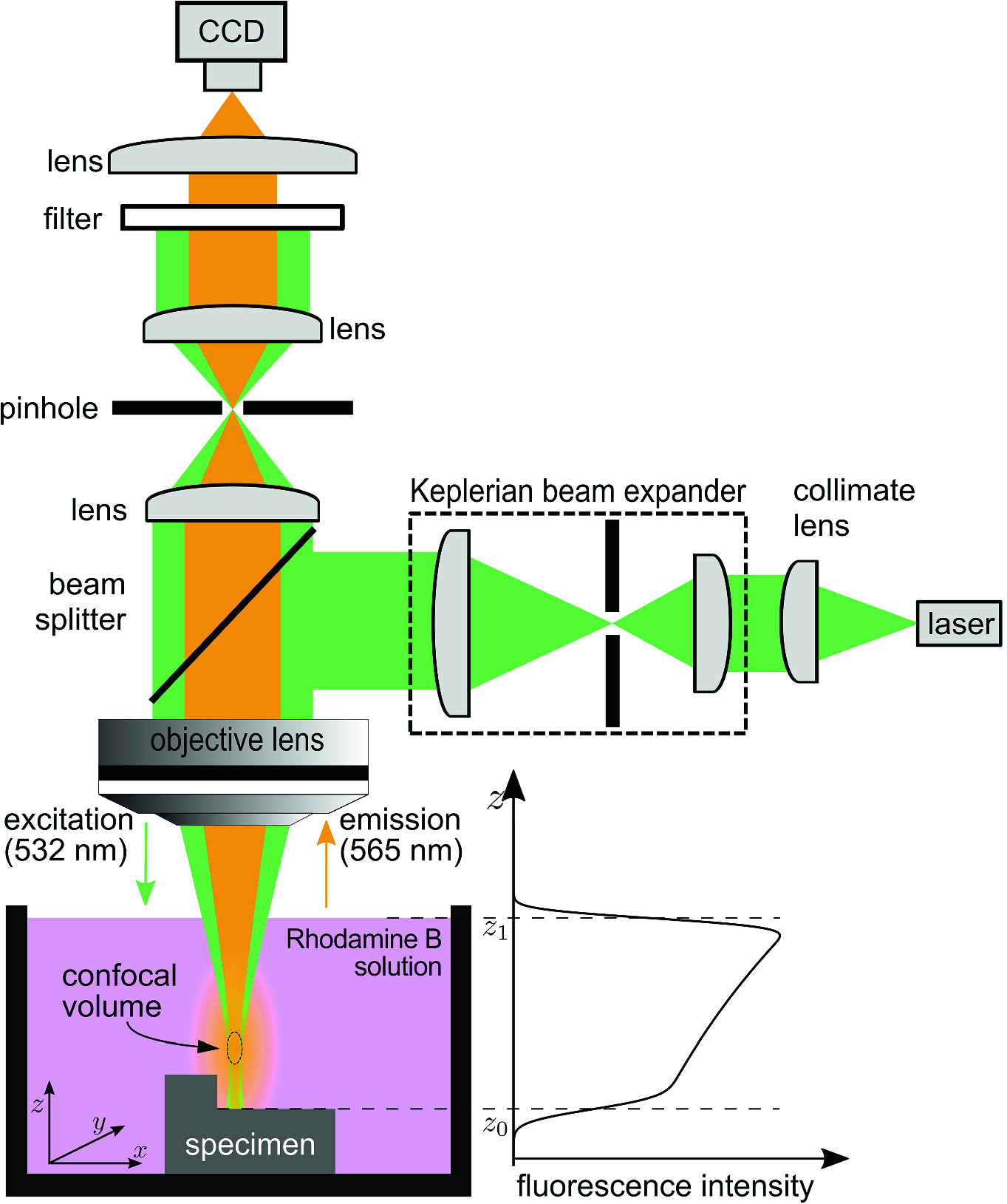
Schematic diagram of the experimental setup and measurement principle of the confocal fluorescence microscopy system. Moving the confocal volume vertically through the fluid, a characteristic fluorescence intensity signal is generated (bottom right) [Mik18]
Since the excitation light is filtered out, only light that is emitted by the fluid inside the confocal volume is detected. Only for values of z inside the boundaries of the fluid (z0 < z < z1, see Fig. 5.24) will a significant signal be produced, since no fluorescent fluid is present to generate light when the confocal volume is fully located in either air or the specimen. The signal does not decay abruptly at the boundary but gradually, depending on the vertical extent of the confocal volume. The exact determination of the surface position z0 is not trivial, as opposed to the case of very thin fluid layers, where the depth response is more similar to that of conventional confocal microscopy where the intensity peak corresponds directly to the surface position. For the case of thicker fluid layers, the properties of the fluorescence signal depend strongly on the fluorophore concentration and the fluid depth. With high fluorophore concentrations or thick fluid layers, the Lambert–Beer law of absorption causes less excitation light to reach far into the fluid, resulting in the decay of the fluorescence signal before the confocal volume reaches the specimen surface. This effect is negligible for thin fluid layers, but needs to be taken into consideration when choosing the fluorophore concentration for measurements in thicker layers. For the purpose of determining the surface position of the specimen from the fluorescence signal, a physical model of the fluorescence signal is used.
5.4.2.1 Model Assumptions
- 1.
The detected fluorescence intensity is only generated in the confocal volume
- 2.
The shape of the confocal volume is simplified to a 3D Gaussian function
- 3.
The shape of the confocal volume is not affected by refraction
- 4.
The specimen surface is non-reflective
- 5.
The fluid surface does not move
- 6.
A constant and uniform fluorophore concentration
- 7.
A constant excitation power
- 8.
The confocal volume is cut off by the horizontal surface element
The model assumptions are the source of model uncertainties that propagate into the uncertainty of the geometry parameter determination. However, it could be shown [Mik18] that even this simplified model is capable of enabling the surface position to be determined within thick fluid layers. The advantage of these simplifications is the existence of a closed mathematical formula to describe the fluorescence intensity signal (see Eq. 5.27).
5.4.2.2 Model Description


 in the xy-direction and
  in the z-direction, where
  is a constant factor dependent on the confocal setup. The parameter
  describes the maximum fluorescence light power determined by the excitation power and fluorophore concentration. Because the signal is generated by scanning the confocal volume through the fluid, a weighting factor, which is zero outside the boundaries of the fluid and follows the Lambert–Beer law of absorption inside the fluorophore, needs to be considered. The fluorescence intensity signal
  detected at position z (see Fig. 5.25) is obtained by integrating the total contribution described by weighting the confocal volume function over all dimensions. The integral over the confocal volume function can be thought of as a vertical (z) convolution of the horizontal (x, y) integral
  with the weighting function
  of the fluid
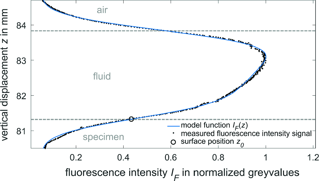


 from Eq. 5.25 gives the model function of the fluorescence intensity signal
  as
as

The surface position  is then determined by a non-linear regression of the measured fluorescence intensity signal with the model function
  using a least squares method. The approximation parameters are the amplitude
  , the offset
  , the fluorophore concentration-dependent attenuation coefficient
  , the confocal volume shape parameter
  and the position parameters
  (fluid surface) and
  (specimen surface).
5.4.3 Experimental Validation
The in situ measurement technique was validated by measuring the geometry parameter step height of a referenced step object [Mik18]. The fluorescence intensity signal resulting from the measurement of a single point on the step-specimen is shown in Fig. 5.25.
 -scan for each
  -point). The surface position
  was determined from each measured intensity signal, with a least-squares approximation using Eq. 5.27. The resulting specimen surface positons
  are shown in Fig. 5.26. After correcting the tilt of the step and the focus shift due to refraction at the fluid surface, the step height
  was determined by the difference of the mean surface positions of each step surface
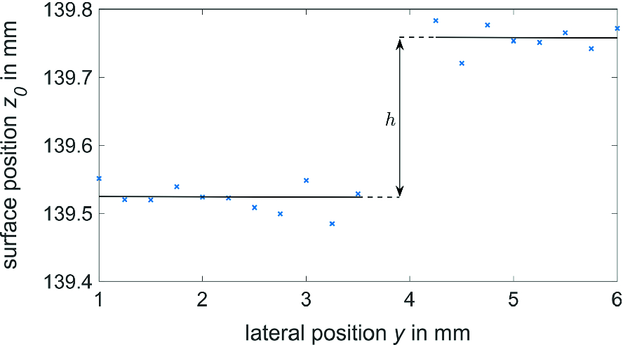
Result of the surface position measurements for the step object. The geometry parameter step height h was determined by the difference of the two mean surface positions of each step surface, resulting in  [Mik18]

Comparing the step height result of  with the tactile reference measurement of
  shows no significant systematic deviations. Since the positions on each step surface show a relatively large stochastic scattering (up to 20%), the uncertainties are most likely caused by the general surface condition or uncertainties in the fitting model. The measurement technique based on confocal fluorescence microscopy was thus shown to be capable of determining the geometry parameter step height for microstructures submerged in thick fluid layers >100
  , which demonstrates the suitability of the model-based approach for in situ application. However, the sources of the uncertainty of
  need to be further characterized in order to reduce it to the desired
  . In order to find the lower boundary of uncertainty for the confocal microscopy-based geometry measurement of submerged micro-structures, a determination of the measurement uncertainty with the approximation of the signal model is necessary.
5.4.4 Uncertainty Characterization
 from the measurement with the non-linear least squares approximation method, the covariance matrix of the estimator
![$$ {\hat{\uptheta }}_{{I_{F} }} = \left[ {{\hat{\text{I}}}_{0} ,{\hat{\text{C}}},\hat{\upepsilon },\hat{\upxi },{\hat{\text{z}}}_{0} ,{\hat{\text{z}}}_{1} } \right]^{T} , $$](../images/463048_1_En_5_Chapter/463048_1_En_5_Chapter_TeX_Equ30.png)
 (see Eq. 5.27) needs to be calculated. Applying an uncertainty propagation calculation to the least squares estimator gives the following relation for the estimator’s covariance matrix [Kay93]:
 denotes the Jacobian matrix with the partial derivatives of the approximation function with respect to
  at each position
  of the measured fluorescence intensity signal
  , and
, and  the covariance matrix whose main diagonal contains the variance
  of each
  of the fluorescence signal
  , since the covariance between the individual values is assumed to be zero.
 of the measurement using the non-linear regression of the model function
  (see. Eq. 5.27), the average variance of the measured fluorescence signal around the model curve, i.e.
  (in units of detected photons), is used. The calculation results in an uncertainty of 8.56 μm for the surface position
  and 3.75 μm if propagated into an uncertainty for the step height (based on 23 surface position measurements, according to the results from Fig. 5.26). The uncertainty of the experimental result of 8.8 μm is still larger than the calculated uncertainty by a factor of 2.3, suggesting varying conditions during the measurement, such as the form of the fluid surface or the micro topography of the specimen. To analyze the effects of the parameters fluid depth
  and concentration-dependent attenuation coefficient
  , the uncertainty
  is determined as a function of the fluid depth
  for different attenuation coefficients
  , shown in Fig. 5.27. The calculation reveals, that for each
  , a fluid depth exists where the uncertainty of the surface position
  is at a minimum (marked as a black cross).
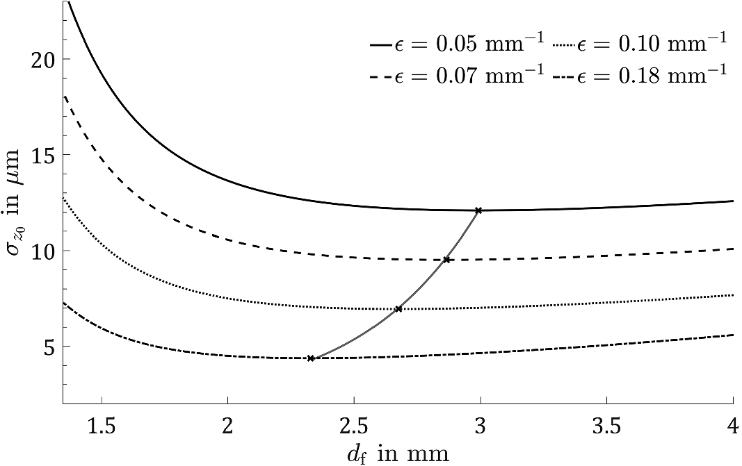
Calculated uncertainty of the surface position  as a function of the fluid depth
  . The minimum uncertainty for each different attenuation coefficient
  is shown as a black cross
The minimum decreases with higher attenuation coefficients  and lower fluid depths
  , which allows a suitable concentration (i.e.
  ) to be chosen for any particular application-dependent fluid depth to achieve optimal uncertainty. A Monte-Carlo (MC) simulation of the surface position determination (fitting an artificial signal with equivalent noise 10,000 times) was used to verify the results of the uncertainty calculations. To determine the theoretical limit of the achievable uncertainty, the variance
  of the fluorescence intensity is decreased to its theoretical minimum. For this, an ideal, shot-noise limited signal with a Poisson distributed variance is considered, resulting in a surface position uncertainty of
  for the 23 position measurements of the experiment (see Fig. 5.26). As a result, the shot-noise limited uncertainty is two orders of magnitude lower than the currently achieved measurement uncertainty. However, if the variance of the fit residuum is considered, the theoretically achievable uncertainty of the surface position for a fluid thickness of
  amounts to
  , which corresponds to a step height uncertainty of
  . These results demonstrate the untapped potential of the measurement technique and suggest that the step height uncertainty of the model-based measurement approach is only limited by the natural variation of the surface or effects not considered in the model (model uncertainties). Hence, a sub-micrometer precision seems feasible with the proposed confocal fluorescence microscopy technique, if the model uncertainties are decreased and the signal-to-noise ratio is maximized in future investigations.
Acknowledgements The editors and authors of this book like to thank the Deutsche Forschungsgemeinschaft DFG (German Research Foundation) for the financial support of the SFB 747 “Mikrokaltumformen—Prozesse, Charakerisierung, Optimierung” (Collaborative Research Center “Micro Cold Forming—Processes, Characterization, Optimization”). We also like to thank our members and project partners of the industrial working group as well as our international research partners for their successful cooperation.
5.5 Characterization of Semi-finished Micro Products and Micro Components
Bernd Köhler, Brigitte Clausen* and Hans-Werner Zoch
Abstract The mechanical properties of semi-finished micro products and micro components cannot easily be extrapolated from macro material. The effects of microstructure and surface conditions have a strong influence on the reliability of measuring results and on the material properties. To evaluate new approaches in micro wire and foil production new testing techniques had to be applied. Furthermore, the suitability of bonding techniques in production processes had to be tested dynamically. Finally, the mechanical properties of micro components produced with the newly developed techniques had to be validated.
Keywords Microstructure · Tensile strength · Fatigue
5.5.1 Introduction
Acquiring the mechanical properties of micro samples demands additional awareness concerning the effects of microstructure, surface, and alignment influences. In both tensile and fatigue tests of thin sheets, the edges of samples have to be very smooth and without micro notches to prevent them from early failure [Köh10b]. It is even more important to observe a correct alignment of the samples than for common samples, since eccentricity in the driving direction can lead to wrinkling and accelerate failure [Hon03]. Frames to place them into the testing device [Hon03] can additionally support especially sensitive samples. The ratio between the sample dimensions and the spatial extent of micro structural features causes size effects on, for example, the yield strength.
The strongest influence is caused by the inhibition of dislocation movement due to surface effects and a lack of dislocation sources. For sample sizes between 1 and 10 µm, this effect causes a strong increase of the yield strength. Furthermore, strain gradient plasticity effects influence the yield strength, due to additionally generated geometrically necessary dislocations (GND). Assuming a length scale of possible interactions with mobile dislocations between 10 nm and 100 µm, the plastic deformation in micro samples can be described satisfactorily [Vol09]. The surface grain model [Kal96] takes into account the difference between the influence of the surface grains and the influence of core grains on the yield strength. The plastic deformation of surface grains occurs more easily than for core grains due to a smaller contribution to strain hardening. The effect is measureable in sample sizes less than 20 times the average grain size [Kal96]. Among the different approaches to calculation, Köhler et al. [Köh13] summarized the yield strength dependencies from structural features. They show that for micro metal forming applications, the temperature and strain rate dependence on the yield strength can be neglected. For samples with less than 20 grains in the cross-section, an increasing yield strength effect in comparison to single crystals occurs due to the different orientation of grains towards the applied stress and the lack of strain continuity across grain boundaries. The increase can be calculated by a crystal orientation factor mor [Tay56]. For samples with more than 20 grains in the cross-section, the Hall–Petch relation works well to calculate the grain size influence. An additional term taking the grain boundary resistance (GBR) into account effects a further increase of yield strength. Kim et al. [Kim07], using an extended Hall–Petch relation, provided a combination of both.
Since the local microstructure gains a higher influence on the mechanical properties, the natural scatter in the local microstructure results in larger scatter in the mechanical properties (see Sect. 1.4.2.2 Scatter).
5.5.2 Equipment for Testing Micro Samples
5.5.2.1 Mechanical Testing

Clamping device used for the quasi-static and cyclic testing of wires
Ultra-micro hardness measurements on the rotary swaged wires made of 304 stainless steel showed that they undergo a strong work hardening due to the forming process and have a surface hardness up to 550 HV 0.03 [Köh17]. To ensure a satisfactory endurance of the rollers, a nitriding steel (31CrMoV9) was chosen as material. After manufacturing, the rolls were quenched and tempered (870 °C 2 h/oil/550 °C 2 h) and nitrided (510 °C 24 h) up to a nitriding depth of about 0.3 mm. A surface hardness of 900 HV 0.1 or 65 HRC, respectively, was achieved.
5.5.2.2 Metallographic Investigations
The change of microstructure due to deformation and heat treatment has to be documented and interpreted to understand the mechanisms occurring in micro cold forming. Besides classic metallographic methods, an electron backscatter scanning diffractometer (EBSD) was used to obtain the grain sizes in aluminum sheets, recognize the anisotropic microstructure, and scan the phase distribution. For this purpose, a Philips XL30 scanning electron microscope (SEM) with an EBSD detector EDAX DigiView IV was available. The sample preparation for optimized EBSD imaging was dependent on the material to be analyzed. To avoid misinterpretation due to preparation failures, an investigation of the influence of different preparation techniques on the results of the EBSD micrographs was started. The results were published by Köhler et al. [Köh18].
5.5.3 Tensile Tests on Micro Samples
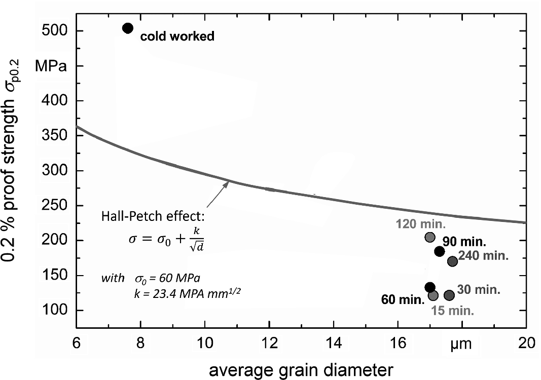
0.2% yield strength of DC01 sheets in dependence on heat treatment and grain diameter compared to the theoretical yield strength due to Hall–Petch relation. The cold worked sheets were annealed at 850 °C in a salt bath for the given time [Köh10a]

 and
and  in the Hall–Petch relation are extended by the hardness-dependent contribution
  (see Eqs. 5.32 and 5.33), wherein c is a material-dependent parameter. A hardness of 150 HV is assumed for the soft annealed state of the mild steel. The differing grain sizes d and grain boundaries resistances of surface and core grains, ksurface and kcore, as well as the friction stress σ0 are explicitly taken into account:


With this newly developed relation, the dependence of the 0.2% yield strength of micro sheets on the grain size could be predicted with a satisfactory accuracy [Köh11a].
The characterization of the first thin films generated by physical vapor deposition required the simultaneous consideration of the test result and the microstructure [Sto10]. Typical deposition effects, like hillocks, explained the unusually high differences in the results of nominally equal batches. The enhancement of the process quality resulted in more homogeneous tensile test results, suitable to adjust the process parameters of the sputter process [Kov17].
A customized clamping technique for micro wires was successfully applied on the incrementally forged samples. As expected, the specimen failure occurred predominantly within the gauge length. In the tensile test results, the scatter was tolerable, though the results were sometimes unexpected.

0.2% yield strength σp0.2 and ultimate tensile strength σu of rotary swaged micro wires produced from 304 stainless steel as a function of feed rate [Köh17]
5.5.4 Endurance Tests on Micro Samples
Woehler diagram of rotary swaged micro wires produced from 304 stainless steel for varied feed rates supplemented by calculated failure probabilities PF (● = run out, ○ = failure) [Köh17]
Fraction of failure occurrence in surface, volume and at non-metallic inclusions of the dynamically tested rotary swaged micro wires produced from 304 stainless steel
Initial state (%) | 1 mm/s (%) | 3 mm/s (%) | 5 mm/s (%) | |
|---|---|---|---|---|
Surface | 0 | 20 | 27 | 22 |
Inclusion | 12 | 10 | 15 | 0 |
Volume | 88 | 70 | 58 | 78 |

Superposition of micrographs (with martensite proof etchant), position of failures with highest probability, and hardness curves of rotary swaged micro wires produced from 304 stainless steel for different feed rates (feed rate from left to right: 1, 3, and 5 mm/s) [Köh17]

Residual stresses in the surface of rotary swaged micro wires produced from 304 stainless steel with a feed rate of 5 mm/s
5.5.5 Microstructure Analysis with EBSD on Rotary Swaged Samples

Image quality (left) and EBSD image (right) of 304 stainless steel wire microstructure in the initial state
Image quality (left) and EBSD image (right) of 304 stainless steel wires microstructure in rotary swaged state with degree of deformation φ = −1.46
Acknowledgements The editors and authors of this book like to thank the Deutsche Forschungsgemeinschaft DFG (German Research Foundation) for the financial support of the SFB 747 “Mikrokaltumformen—Prozesse, Charakerisierung, Optimierung” (Collaborative Research Center “Micro Cold Forming—Processes, Characterization, Optimization”). We also like to thank our members and project partners of the industrial working group as well as our international research partners for their successful cooperation.

Open Access This chapter is licensed under the terms of the Creative Commons Attribution 4.0 International License (http://creativecommons.org/licenses/by/4.0/), which permits use, sharing, adaptation, distribution and reproduction in any medium or format, as long as you give appropriate credit to the original author(s) and the source, provide a link to the Creative Commons license and indicate if changes were made.
The images or other third party material in this chapter are included in the chapter's Creative Commons license, unless indicated otherwise in a credit line to the material. If material is not included in the chapter's Creative Commons license and your intended use is not permitted by statutory regulation or exceeds the permitted use, you will need to obtain permission directly from the copyright holder.