Chapter 3

Linear Algebra

This chapter contains some very basic and some relatively advanced material, which is needed only in a few later chapters. Hence, it can be read in quite different ways, depending on readers’ interest:

• Readers interested in elementary probability and statistics (Chapters 4–11) may just have a look at Sections 3.1 and 3.2, which motivate and illustrate basic approaches to solve systems of linear equations; this is an important topic that any reader should be familiar with.
• The remaining sections of this chapter are more advanced, but they are mostly needed by those interested in the multivariate statistics techniques described in Chapters 15–17. One possibility is reading this whole chapter now; alternatively, one might prefer just having a cursory look at the material, and returning here when tackling those chapters.
• Finally, readers who are interested in optimization modeling can do the same when grappling with Chapter 12. Some concepts related to quadratic forms (Section 3.8) and multivariable calculus (Section 3.9) are useful to obtain a better grasp of some technical aspects of optimization. Apparently, these are not necessary if you are just interested in building an optimization model, but not in the algorithms needed to solve it; nevertheless, an appreciation of what a convex (i.e., easy-to-solve) optimization model is better gained if you are armed with the background we build here.

In Section 3.1 we propose a simple motivating example related to pricing a financial derivative. A simple binomial valuation model is discussed, which leads to the formulation of a system of linear equations. Solving such a system is the topic of Section 3.2, where we disregard a few complicating issues and cut some corners in order to illustrate standard solution approaches. In Sections 3.3 and 3.4 we move on to more technical material: vector and matrix algebra. Matrices might be new to some readers, but they are a ubiquitous concept in applied mathematics. On the contrary, you are likely to have some familiarity with vectors from geometry and physics. We will abstract a little in order to pave the way for Section 3.5, dealing with linear spaces and linear algebra, which can be considered as a generalization of the algebra of vectors. Another possibly familiar concept from elementary mathematics is the determinant, which is typically taught as a tool to solve systems of linear equations. Actually, the concept has many more facets, and a few of them are dealt with in Section 3.6. The last concepts from matrix theory that we cover are eigenvalues and eigenvectors, to which Section 3.7 is devoted. They are fundamental, e.g., in data reduction methods for multivariate statistical analysis, like principal component analysis and factor analysis.1 The two last sections are, in a sense, halfway between linear algebra and calculus. In Section 3.8 we consider quadratic forms, which play a significant role in both statistics and optimization. They are, essentially, the simplest examples of a nonlinear function of multiple variables, and we will consider some of their properties, illustrating the link between eigenvalues of a matrix and convexity of a function. Finally, in Section 3.9 we hint at some multivariable generalizations of what we have seen in the previous chapter on calculus for functions of a single variable.

3.1 A MOTIVATING EXAMPLE: BINOMIAL OPTION PRICING

Options are financial derivatives that have gained importance, as well as a bad reputation, over the years. In Section 1.3.1 we considered forward contracts, another type of derivative. With a forward contract, two parties agree on exchanging an asset or a commodity, called the underlying asset, at a prescribed time in the future, for a fixed price determined now. In a call option, one party (the option holder, i.e., the party buying the option) has the right but not the obligation to buy the asset from the other party (the option writer, i.e., the party selling the option) at a price established now. This is called the strike price, which we denote by K. Let us denote the current price of the underlying asset by S0 (known when the option is written) and the future price at a time t = T by ST. Note that ST, as seen at time t = 0, is a random variable; the time t = T corresponds to the option maturity, which is when the option can be exercised.2 Clearly, the option will be exercised only if ST ≥ K, since there would be no point in using the option to buy at a price that is larger than the prevailing market price at time T. Then the payoff of the option, for the holder, is

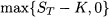
To interpret this, consider the possibility of exercising the option to buy at K an asset that can be immediately sold at ST. Market structure is not really that simple, but some options are settled in cash, so the payoff really has a monetary nature; this occurs for options written on a nontraded market index or on interest rates. This payoff is a piecewise linear function and is illustrated in Fig. 3.1. When the future asset price ST will be realized, at time t = T, the payoff will be clearly determined. What is not that clear is the fair price for the contract at time t = 0: The payoff for the option holder cannot be negative, but the option writer can suffer a huge loss; hence, the latter requires an option premium, paid at time t = 0, to enter into this risky contract. Here we consider the most elementary model for option pricing. Whatever model we may think of, it should account for uncertainty in the price of the underlying asset, and the simplest model of uncertainty is a binomial model.3 As shown in Fig. 3.2, a binomial model for the price of the underlying asset assumes that its price in the future can take one of two values. It is quite common in financial modeling to represent uncertainty using multiplicative shocks, i.e., random variables by which the current stock price is multiplied to obtain the new price. In a binomial model, this means that the current price S0, after a time period of length T, is multiplied by a shock that may take values d or u, with probabilities pu and pd, respectively. It is natural to think that d is the shock if the price goes down, whereas u is the shock when the price goes up; so, we assume d < u. The asset price may

Fig. 3.1 Payoff of a call option.

Fig. 3.2 One-step binomial model for option pricing.

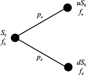
be either S0u or S0d, and the option will provide its holder a payoff fu and fd corresponding to the two outcomes. These values are also illustrated in Fig. 3.2. For instance, in the case of a call option with strike price K, we have

The pricing problem consists of finding a fair price f0 for the option, i.e., its value at time t = 0. Intuitively, one would guess that the two probabilities pu and pd play a major role in determining f0. Furthermore, individual risk aversion could also play a role. Different people may assign a different value to a lottery, possibly making the task of finding a single fair price a hopeless endeavor, unless we have an idea of the aggregate risk aversion of the market as a whole.

However, a simple principle can be exploited in order to simplify our task. The option is a single, somewhat complicated, asset; now suppose that we are able to set up a portfolio of simpler assets, in such a way that the portfolio yields the same payoff as the option, in any possible future state. The value of this replicating portfolio at t = 0 is known, and it cannot differ from the option value f0. Otherwise, there would be two essentially identical assets traded at different prices. Such a violation of the law of one price would open up arbitrage opportunities.4

The replicating portfolio should certainly include the underlying asset, but we need an additional one. Financial markets provide us with such an asset, in the form of a risk-free investment. We may consider a bank account yielding a risk-free interest rate r; we assume here that this rate is continuously compounded,5 so that if we invest $1 now, we will own $ert at a generic time instant t. Equivalently, we may think of a riskless zero-coupon bond, with initial price B0 = 1 and future price B1 = erT, when the option matures at time t = T.

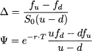
What we have to find is the number of stock shares and riskless bonds that we should include in the portfolio, in order to replicate the option payoff. Let us denote the number of stock shares by Δ and the number of bonds by Ψ. The initial value of this portfolio is

(3.1)

and its future value, depending on the realized state, will be either

Note that future value of the riskless bond does not depend on the realized state. If this portfolio has to replicate the option payoff, we should enforce the following two conditions:

(3.2)

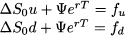
This is a system of two linear equations in two unknown variables Δ and Ψ. The equations are linear as variables occur linearly. There is no power like x3, or cross-product like x1 ˙ x2, or any weird function involved. All we have to do is solve this system of linear equations for Δ and Ψ, and plug the resulting values into Eq. (3.1) to find the option price f0. A simple numerical example can illustrate the idea.

Example 3.1 Let us assume that option maturity is T = 1 year, the risk-free interest rate is 10%, the current price of the stock share is $10, and the strike price is $11. Finally, say that the two possible returns of the stock share in one year are either 20% or -10%, which imply u = 1.2 and d = 0.9. The corresponding payoffs are

The system of linear equations is

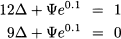
If we subtract the second equation from the first one, we get

Plugging this value back into the first equation yields

and putting everything together, we obtain

Note that a negative value of Ψ means that we borrow some money, at the risk-free rate.

To get a financial understanding of what is going on, you should take the point of view of the option writer, i.e., the guy selling the option. Say that he takes a “naked” position, i.e., he collects the option price and waits until maturity. If the stock price goes up, he will have to buy one share at $12 just to hand it over to the option holder for $11, losing $1. If he does not like taking this chance, he could consider the opposite position: Buy one stock share, just in case the option gets exercised by its holder. This “covered” position does not really solve the problem, as the writer loses $1 if the price goes down, the option is not exercised, and he has to sell for $9 the share that was purchased for $10.

The replicating strategy suggests that, to hedge the risk away, the writer should actually buy Δ = 1/3 shares. To this aim, he should use the option premium, plus some borrowed money ($2.7145, as given by Ψ). If the stock price goes down to $9, the option writer will just sell that share for $3, i.e., what he needs to repay the debt, which at the risk-free rate has risen to $3. Hence, the option writer breaks even in the “down” scenario. The reader is encouraged to work out the details for the other case, which requires purchasing two additional thirds of a stock share at the price of $12, in order to sell a whole share to the option holder, and to verify that the option writer breaks even again (in this case, the proceeds from the sale of the share at the strike price are used to repay the outstanding debt).

This numerical example could leave the reader a bit puzzled: Why should anyone write an option just to break even? No one would, of course, and the fair option price is increased somewhat to compensate the option writer. Furthermore, we have not considered issues such as transaction costs incurred when trading stock shares. Most importantly, the binomial model of uncertainty is oversimplified, yet it does offer a surprising insight: The probabilities pu and pd of the up/down shocks do not play any role, and this implies that the expected price of the stock share at maturity is irrelevant. This is not surprising after all, as we have matched the option payoff in any possible state, irrespective of its probability. Moreover, the careful reader will recall that we reached a similar conclusion when dealing with forward contracts in Section 1.3.1. There, by no-arbitrage arguments that are actually equivalent to what we used here, it was found that the fair forward price for delivery in one year is F0 = S0(1 + r), where S0 is the price of the underlying asset at time t = 0 and r is the risk-free rate with annual compounding. In the case of continuous compounding and generic maturity T, we get F0 = S0erT.

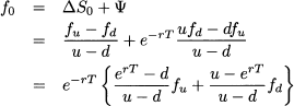
Let us try to see if there is some link between forward and option pricing. To begin with, let us solve the system of linear equations (3.2) in closed form. Using any technique described in the following section,6 we get the following composition of the replicating portfolio:

Hence, by the law of one price, the option value now is

(3.3)

As we already noticed, this relationship does not depend on the objective probabilities pu and pd. However, let us consider the quantities

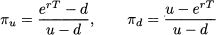
which happen to multiply the option payoffs in Eq. (3.3). We may notice two interesting features of πu and πd:

1. They add up to one, i.e., πu + πd = 1.

2. They are nonnegative, i.e., πu, πd ≥ 0, provided that d ≤ erT ≤ u.

The last condition does make economic sense. Suppose, for instance, that erT < d < u. This means that, whatever the realized scenario, the risky stock share will perform better than the risk-free bond. But this cannot hold in equilibrium, as it would pave the way for an arbitrage: Borrow money at the risk-free rate, buy the stock share, and you will certainly be able to repay the debt at maturity, cashing in the difference between the matured debt and the stock price. On the contrary, if the risk-free rate is always larger than the stock price in the future, one could make easy money by selling the stock share short.7

We already know that probabilities may be related to relative frequencies and that the latter do add up to one and are nonnegative. Then we could interpret πu and πd as probabilities and Eq. (3.3) can be interpreted in turn as the discounted expected value of the option payoff

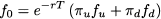
provided that we do not use the “objective” probabilities pu and pd, but πu and πd. These are called risk-neutral probabilities, a weird name that we can easily justify. Indeed, if we use the probabilities πu and πd, the expected value of the underlying asset at maturity is

where the notation E emphasizes that change in probability measure.8 This suggests that, under these unusual probabilities, the return of the risky asset is just the risk-free return. Furthermore, this is just the forward price of the underlying asset. In other words, the forward price is in fact the expected value of the underlying asset, but under modified probabilities. But how is it possible that the expected return of a risky asset is just the risk-free rate? This might happen only in a world where investors do not care about risk, i.e., in a risk-neutral world, which justifies the name associated with the probabilities we use in option pricing. Indeed, what we have just illustrated is the tip of a powerful iceberg, the risk-neutral pricing approach, which plays a pivotal role in financial engineering.

Of course, the binomial model we have just played with is too simple to be of practical use, but it is the building block of powerful pricing methods. We refer the interested reader to references at the end of this chapter, but now it is time to summarize what we have learned from a general perspective:

• Building and solving systems of linear equations may be of significant practical relevance in many domains, including but not limited to financial engineering. We have already stumbled on systems of linear equations when solving the optimal production mix problem in Section 1.1.2.
• We have also seen an interplay between algebra and probability theory; quantitative, fact-based business management requires the ability of seeing these and other connections.
• We have considered a simple binomial model of uncertainty. We had two states, and we used two assets to replicate the option. What if we want a better model with three or more states? How many equations do we need to find a solution? More generally, under which conditions are we able to find a unique solution to a system of linear equations?

We will not dig deeper into option pricing, which is beyond the scope of the book, but these questions do motivate further study, which is carried out in the rest of this chapter. But first, we should learn the basic methods for solving systems of linear equations.

3.2 SOLVING SYSTEMS OF LINEAR EQUATIONS

The theory, as well as the computational practice, of solving systems of linear equations is relevant in a huge list of real-life settings. In this section we just outline the basic solution methods, without paying due attention to bothering issues such as the existence and uniqueness of a solution, or numerical precision.

A linear equation is something like

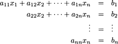
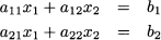
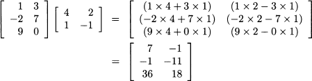
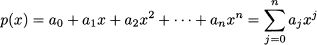
i.e., it relates a linear function of variables x1, …, xn to a right-hand side b. A system of linear equations involves m such equations:

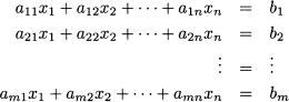
where aij is the coefficient multiplying variable xj, j = 1, …, n, in equation i, i = 1, …, m, whose right-hand side is bi.

A preliminary question is: How many equations should we have to pinpoint exactly one solution? An intuitive reasoning about degrees of freedom suggests that we should have as many equations as unknown variables. More precisely, it seems reasonable that

• If we have more variables than equations (n > m), then we may not find one solution, but many; in other words, we have an underconstrained problem, and the residual degrees of freedom can be exploited to find a “best” solution, possibly optimizing some cost or profit function, much along the lines of Section 1.1.2; we will see how to take advantage of such cases in Chapter 12 on optimization modeling.
• If we have more equations than variables (n < m), then we may fail to find any solution, as the problem is overconstrained; still, we might try to find an assignment of variables such that we get as close as possible to solving the problem; this leads to linear regression models and the least-squares method (see Chapter 10).
• Finally, if n = m, we may hope to find a unique solution.

Actually, this straightforward intuition will work in most cases, but not always. This is easy to visualize in a two-dimensional space, as illustrated in Fig. 3.3. In such a setting, a linear equation like a1x1 + a2x2 = b corresponds to a line (see Section 2.3). In case (a), we have one equation for two unknown variables; there are infinite solutions, lying on the line pinpointed by the equation. If we have two equations, as in case (b), the solution is the unique point where the two lines intersect. However, if we have three lines as in case (c), we may fail to find a solution, because three lines have no common intersection, in general. These cases correspond to our intuition above. Nevertheless, things can go wrong. In case (d), we have two lines, but they are parallel and there is no solution. To see an example, consider the system

Fig. 3.3 Schematic representation of issues in existence and uniqueness of the solution of systems of linear equations.

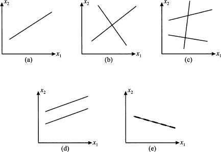
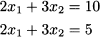
If we subtract the second equation from the first one, we get 0 = 5, which is, of course, not quite true. By a similar token, in case (e) we have two equations, but the solution is not unique. Such a case may arise when two apparently different equations boil down to the same one, as in the following system:

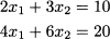
It is easy to see that the two equations are not really independent, since the second one is just the first one multiplied by 2.

Indeed, to address issues related to existence and uniqueness of solutions of systems of linear equations, we need the tools of linear algebra, which we cover in the advanced sections of this chapter. The reader interested in a basic treatment might just skip these sections. Here, we illustrate the basic approaches to solve systems of linear equations, assuming that the solution is unique, and that we have as many equations as variables.

3.2.1 Substitution of variables

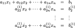
A basic (highschool) approach to solving a system of linear equations is substitution of variables. The idea is best illustrated by a simple example. Consider the following system:

(3.4)

Rearranging the first equation, we may express the first variable as a function of the second one:

and plug this expression into the second equation:

Then we may plug this value back into the expression of x1, which yields x1 = 2.

Despite its conceptual simplicity, this approach is somewhat cumbersome, as well as difficult to implement efficiently in computer software. A related idea, which is more systematic, is elimination of variables. In the case above, this is accomplished as follows:

1. Multiply the first equation by -3, to obtain -3x1 + 6x2 = -24

2. Add the new equation to the second one, which yields 7x2 = -21 and implies x2 = - 3

3. Substitute back into the first equation, which yields x1 = 2

We see that elimination of variables, from a conceptual perspective, is not that different from substitution. One can see the difference when dealing with large systems of equations, where carrying out calculations without due care can result in significant numerical errors. Gaussian elimination is a way to make elimination of variables systematic.

3.2.2 Gaussian elimination

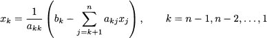
Gaussian elimination, with some improvements, is the basis of most numerical routines to solve systems of linear equations. Its rationale is that the following system is easy to solve:

Such a system is said to be in upper triangular form, as nonzero coefficients form a triangle in the upper part of the layout. A system in upper triangular form is easy to solve by a process called backsubstitution. From the last equation, we immediately obtain

Then, we plug this value into the second-to-last (penultimate) equation:

In general, we proceed backward as follows:

(3.5)

Now, how can we transform a generic system into this nice triangular form? To get a system in triangular form, we form combinations of equations in order to eliminate some coefficients from some equations, according to a systematic pattern. Starting from the system in its original form

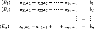
where (Ek) denotes the kth equation, k = 1, …, n, we would like to get an equivalent system featuring a column of zeros under the coefficient a11. By “equivalent” system we mean a new system that has the same solution as the first one. If we multiply equations by some number, we do not change their solution; by the same token, if we add equations, we do not change the solution of the overall system.

For each equation (Ek) (k = 2, …, n), we must apply the transformation

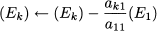
which leads to the equivalent system:

Now we may repeat the procedure to obtain a column of zeros under the coefficient a22(1), and so on, until the desired form is obtained, allowing for backsubstitution. The idea is best illustrated by a simple example.

Example 3.2 Consider the following system:

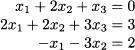
It is convenient to represent the operations of Gaussian elimination in a tabular form, which includes both the coefficients in each equation and the related right-hand side:

It is easy to apply backsubstitution to this system in triangular form, and we find x3 = 1, x2 = -1, and x1 = 1.

Gaussian elimination is a fairly straightforward approach, but it involves a few subtle issues:

1. To begin with, is there anything that could go wrong? The careful reader, we guess, has already spotted a weak point in Eq. (3.5): What if akk = 0? This issue is easily solved, provided that the system admits a solution. We may just swap two equations or two variables. If you prefer, we might just swap two rows or two columns in the tabular form above.

2. What about numerical precision if we have a large-scale system? Is it possible that small errors due to limited precision in the calculation creep into the solution process and ultimately lead to a very inaccurate solution? This is a really thorny issue, which is way outside the scope of the book. Let us just say that state-of-the-art commercial software is widely available to tackle such issues in the best way, which means avoiding or minimizing the difficulty if possible, or warning the user otherwise.

3.2.3 Cramer’s rule

As a last approach, we consider Cramer’s rule, which is a handy way to solve systems of two or three equations. The theory behind it requires more advanced concepts, such as matrices and their determinants, which are introduced below. We anticipate here a few concepts so that readers not interested in advanced multivariate statistics can skip the rest of this chapter without any loss of continuity.

In the previous section, we have seen that Gaussian elimination is best carried out on a tabular representation of the system of equations. Consider a system of two equations in two variables:

We can group the coefficients and the right-hand sides into the two tables below:

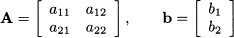
These “tables” are two examples of a matrix, A is a two-row, two-column matrix, whereas b has just one column. Usually, we refer to b as a column vector (see next section).

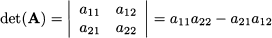
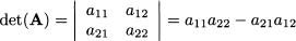
The determinant is a function mapping a square matrix, i.e., a matrix with the same number of rows and columns, to a number. The determinant of matrix A is denoted by det(A) or |A|. The concept is not quite trivial, but computing the determinant for a 2 x 2 matrix is easy. For the matrix above, we have

In practice, we multiply numbers on the main diagonal of the matrix and we subtract the product of numbers on the other diagonal. Let us denote by Bi the matrix obtained by substituting column i of matrix A with the vector b of the right-hand sides. Cramer’s rule says that the solution of a system of linear equations (if it exists) is obtained by computing

(3.6)

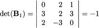
Example 3.3 To illustrate, let us consider system (3.4) again. We need the following determinants:

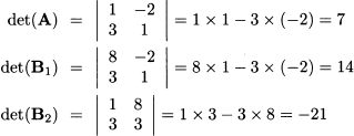
Applying Cramer’s rule yields

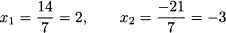
which is, of course, what we obtained by substitution of variables.

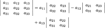
The case of a 3 x 3 matrix is dealt with in a similar way, by computing the determinant as follows:

In general, the calculation of an n x n determinant is recursively boiled down to the calculation of smaller determinants.

Example 3.4 To illustrate the calculation of the determinant in a three-dimensional case, let us apply the formula to the matrix of coefficients in Example 3.2 above:

The reader is encouraged to compute all of the determinants, such as

that we require to apply Cramer’s rule and check that we obtain the same solution as in Example 3.2.9

We will generalize this rule and say much more about the determinant in Section 3.6. We will also see that, although computing the determinant is feasible for any square matrix, this quickly becomes a cumbersome approach. Indeed, determinants are a fundamental tool from a conceptual perspective, but they are not that handy computationally. Still, it will be clear from Section 3.6 how important they are in linear algebra.

For now, we should just wonder if anything may go wrong with the idea. Indeed, Cramer’s rule may crumble down if det(A) = 0. We will see that in such a case the matrix A suffers from some fundamental issues, preventing us from being able to solve the system. In general, as we have already pointed out, we should not take for granted that there is a unique solution to a system of linear equations. There could be none, or there could be many (actually, infinite). To investigate these issues, we need to introduce powerful and far-reaching mathematical concepts related to vectors, matrices, and linear algebra.

3.3 VECTOR ALGEBRA

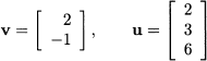
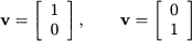
Vectors are an intuitive concept that we get acquainted with in highschool mathematics. In ordinary two- and three-dimensional geometry, we deal with points on the plane or in the space. Such points are associated with coordinates in a Cartesian reference system. Coordinates may be depicted as vectors, as shown in Fig. 3.4; in physics, vectors are associated with a direction (e.g., of motion) or an intensity (e.g., of a force). In this book, we are interested in vectors as tuples of numbers. The vectors of Fig. 3.4 can be represented numerically as a pair and a triple of numbers, respectively:

Fig. 3.4 Vectors in two- and three-dimensional spaces.

More generally, we define a vector in an n-dimensional space as a tuple of numbers:

As a notational aid, we will use boldface lowercase letters (e.g., a, b, x) to refer to vectors; components (or elements) of a vector will be referred to by lowercase letters with a subscript, such as y1 or vi. In this book, components are assumed to be real numbers; hence, an n-dimensional vector v belongs to the set n of tuples of n real numbers. If n = 1, i.e., the vector boils down to a single number, we speak of a scalar element.

Note that usually we think of vectors as columns. Nothing forbids the use of a row vector, such as

In order to stick to a clear convention, we will always assume that vectors are column vectors; whenever we insist on using a row vector, we will use the transposition operator, denoted by superscript T, which essentially swaps rows and columns:

Sometimes, transposition is also denoted by v’.

In business applications, vectors can be used to represent several things, such as

• Groups of decision variables in a decision problem, such as produced amounts xi for items i = 1, …, n, in a production mix problem
• Successive observations of a single random variable X, as in a random sample (X1, X2, …, Xm)
• Attributes of an object, measured according to several criteria, in multivariate statistics

3.3.1 Operations on vectors

We are quite used to elementary operations on numbers, such as addition, multiplication, and division. Not all of them can be sensibly extended to the vector case. Still, we will find some of them quite useful, namely:

• Vector addition
• Multiplication by a scalar
• Inner product

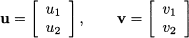
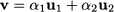
Vector addition Addition is defined for pairs of vectors having the same dimension. If v, u n, we define:

For instance

Since vector addition boils down to elementwise addition, it enjoys commutativity and associativity:

and we may add an arbitrary number of vectors by just summing up their elements.

We will denote by 0 (note the boldface character) a vector whose elements are all 0; sometimes, we might make notation a bit clearer by making the number of elements explicit, as in 0n. Of course, u + (-u) = 0.

Multiplication by a scalar Given a scalar α and a vector v n, we define the product of a vector and a scalar:

For instance

Again, familiar properties of multiplication carry over to multiplication by a scalar.

Now, what about defining a product between vectors, provided that they are of the same dimension? It is tempting to think of componentwise vector multiplication. Unfortunately, this idea does not lead to an operation with properties similar to ordinary products between scalars. For instance, if we multiply two nonzero numbers, we get a nonzero number. This is not the case for vectors. To see why, consider vectors

If we multiply them componentwise, we get the two-dimensional zero vector 02. This, by the way, does not allow to define division in a sensible way. Nevertheless, we may define a useful concept of product between vectors, the inner product.10

Inner product The inner product is defined by multiplying vectors componentwise and summing the resulting terms:

Since the inner product is denoted by a dot, it is also known as the dot product; in other books, you might also find a notation like u, v. The inner product yields a scalar.11 Clearly, an inner product is defined only for vectors of the same dimension. For instance

One could wonder why such a product should be useful at all. In fact, the inner-product concept is one of the more pervasive concepts in mathematics and it has far-reaching consequences, quite beyond the scope of this book. Nevertheless, a few geometric examples suggest why the inner product is so useful.

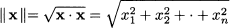
Example 3.5 (Euclidean length, norm, and distance) The inner-product concept is related to the concept of vector length. We know from elementary geometry that the length of a vector is the square root of the sum of squared elements. Consider the two-dimensional vector v = [2, -1]T, depicted in Fig. 3.4. Its length (in the Euclidean sense) is just 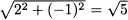. We may generalize the idea to n dimensions by defining the Euclidean norm of a vector:

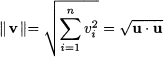
The Euclidean norm || ˙ || is a function mapping vectors to nonnegative real numbers, built on the inner product. Alternative definitions of norm can be proposed, provided that they preserve the intuitive properties associated with vector length. By the same token, we may consider the distance between two points. Referring again to a two-dimensional case, if we are given two points in plane

their Euclidean distance is

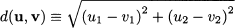
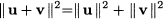
This can be related to the norm and the inner product:

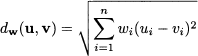
In such a case, we are measuring distance by assigning the same importance to each dimension (component of the difference vector). Later, we will generalize distance by allowing for a vector of weights w, such as in

A vector e such that || e ||= 1 is called a unit vector. Given a vector v, we may obtain a unit vector parallel to v by considering vector v/ || v ||.

Example 3.6 (Orthogonal vectors) Consider the following vectors:

They are unit-length vectors parallel to the two coordinate axes, and they are orthogonal. We immediately see that

The same thing happens, for instance, with v1 = [1, 1]T and v2 = [-1,1]T. These vectors are orthogonal as well (please draw them and check).

Orthogonality is not an intuitive concept in an n-dimensional space, but in fact we may define orthogonality in terms of the inner product: We say that two vectors are orthogonal if their inner product is zero.

Example 3.7 (Orthogonal projection) From elementary geometry, we know that if two vectors u and v are orthogonal, then we must have

This is simply the Pythagorean theorem in disguise, as illustrated in Fig. 3.5. Now consider two vectors u and v that are not orthogonal, as illustrated in Fig. 3.6. We may decompose u in the sum of two vectors, say, u1 and u2, such that u1 is parallel to v and u2 is orthogonal to v. The vector u1 is the orthogonal projection of u on v. Basically, we are decomposing the “information” in u into the sum of two components. One contains the same information as v, whereas the other one is completely “independent.”

Fig. 3.5 Orthogonal vectors illustrating the Pythagorean theorem.

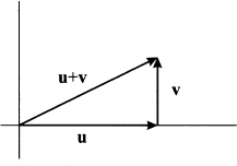
Fig. 3.6 Orthogonal projection of vector u on vector v.

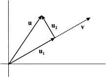
Since u1 is parallel to v, for some scalar a we have:

The first equality derives from the fact that two parallel vectors must be related by a proportionality constant; the second one states that u is the sum of two component vectors. What is the right value of α that makes them orthogonal? Let us apply the Pythagorean theorem:

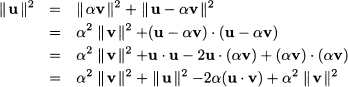
This, in turn, implies

If v is a unit vector, we see that the inner product gives the length of the projection of u on v. We also see that if u and v are orthogonal, then this projection is null; in some sense, the “information” in u is independent from what is provided by v.

3.3.2 Inner products and norms

The inner product is an intuitive geometric concept that is easily introduced for vectors, and it can be used to define a vector norm. A vector norm is a function mapping a vector x into a nonnegative number || x || that can be interpreted as vector length. We have see that we may use the dot product to define the usual Euclidean norm:

It turns out that both concepts can be made a bit more abstract and general, and this has a role in generalizing some intuitive concepts such as orthogonality and Pythagorean theorem to quite different fields.12

Generally speaking, the inner product on a space is a function mapping two elements x and y of that space into a real number x, y. There is quite some freedom in defining inner products, provided our operation meets the following conditions:

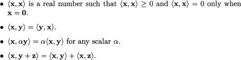
It is easy to check that our definition of the inner product for vectors in n meets these properties. If we define alternative inner products, provided they meet the requirements described above, we end up with different concepts of orthogonality and useful generalizations of Pythagorean theorem. A straightforward generalization of the dot product is obtained by considering a vector w of positive weights and defining:

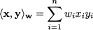
This makes sense when we have a problem with multiple dimensions, but some of them are more important than others.

By a similar token, we may generalize the concept of norm, by requiring the few properties that make sense when defining a vector length:

• || x || ≥ 0, with || x || = 0 if and only if x = 0; this states that length cannot be negative and it is zero only for a null vector.
• || αx || = | α | || x || for any scalar α; this states that if we multiply all of the components of a vector by a number, we change vector length accordingly, whether the scalar is negative or positive.
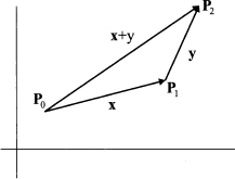
• || x + y || ≤ || x || + || y ||; this property is known as triangle inequality and can be interpreted intuitively by looking at Fig. 3.7 and interpreting vectors as displacement in the plane, and their length as distances. We can move from point P0 to point P1 by the displacement corresponding to vector x, and from point P1 to P2 by displacement y; if we move directly from P0 to P2, the length of the resulting displacement, || x + y ||, cannot be larger than the sum of the two distances || x || and || y ||.

Fig. 3.7 Orthogonal projection of vector u on vector v.

Using the standard dot product, we find the standard Euclidean norm, which can be denoted by || ˙ ||2. However, we might just add the absolute value of each coordinate to define a length or a distance:

(3.7)

The notation is due to the fact that the two norms above are a particular case of the general norm

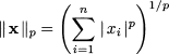
Letting p → +∞, we find the following norm:

(3.8)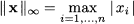

All of these norms make sense for different applications, and it is also possible to introduce weights to assign different degrees of importance to multiple problem dimensions.13

Norms need not be defined on the basis of an inner product, but the nice thing of the inner product is that if we use an inner product to define a norm, we can be sure that we come up with a legitimate norm.

3.3.3 Linear combinations

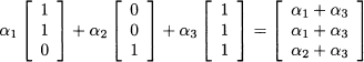
The two basic operations on vectors, addition and multiplication by a scalar, can be combined at wish, resulting in a vector; this is called a linear combination of vectors. The linear combination of vectors vj with coefficients αj, j = 1, …, m is

If we denote each component i, i = 1, …, n, of vector j by vij, the component i of the linear combination above is simply

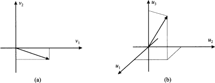
It is useful to gain some geometric intuition to shed some light on this concept. Consider vectors u1 = [1, 1]T and u2 = [-1, 1]T, depicted in Fig. 3.8(a), and imagine taking linear combinations of them with coefficients α1 and α2:

Fig. 3.8 Illustrating linear combinations of vectors.

Which set of vectors do we generate when the two coefficients are varied? Here are a few examples:

The reader is strongly urged to draw these vectors to get a feeling for the geometry of linear combinations. On the basis of this intuition, we may try to generalize a bit as follows:

• It is easy to see that if we let α1 and α2 take any possible value in , we generate any vector in the plane. Hence, we span all of the two-dimensional space 2 by expressing any vector as a linear combination of u1 and u2.
• If we enforce the additional restriction α1, α2 ≥ 0, we take positive linear combinations. Geometrically, we generate only vectors in the shaded region of Fig. 3.8(b), which is a cone.
• If we require α1 + α2 = 1, we generate vectors on the horizontal dotted line in Fig. 3.8(c). Such a combination is called affine combination. Note that in such a case we may express the linear combination using one coefficient α as αu1 + (1 - α)u2. We get vector u1 when setting α = 1 and vector u2 when setting α = 0.
• If we enforce both of the additional conditions, i.e., if we require that weights be nonnegative and add up to one, we generate only the line segment between u1 and u2. Such a linear combination is said a convex combination and is illustrated in Fig. 3.8(d).14

3.4 MATRIX ALGEBRA

We began this chapter by considering the solution of systems of linear equations. Many issues related to systems of linear equations can be addressed by introducing a new concept, the matrix. Matrix theory plays a fundamental role in quite a few mathematical and statistical methods that are relevant for management.

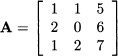
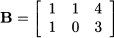
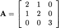
We have introduced vectors as one-dimensional arrangement of numbers. A matrix is, in a sense, a generalization of vectors to two dimensions. Here are two examples of matrices:

In the following, we will denote matrices by boldface, uppercase letters. A matrix is characterized by the number of rows and the number of columns. Matrix A consists of three rows and three columns, whereas matrix B consists of two rows and four columns. Generally speaking, a matrix with m rows and n columns belongs to a space of matrices denoted by m,n. In the two examples above, A 3,3 and B 2,4. When m = n, as in the case of matrix A, we speak of a square matrix.

It is easy to see that vectors are just a special case of a matrix. A column vector belongs to space n,1 and a row vector is an element of 1,n.

3.4.1 Operations on matrices

Operations on matrices are defined much along the lines used for vectors. In the following, we will denote a generic element of a matrix by a lowercase letter with two subscripts; the first one refers to the row, and the second one refers to the column. So, element aij is the element in row i, column j.

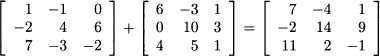
Addition Just like vectors, matrices can be added elementwise, provided they are of the same size. If A m,n and B m,n, then

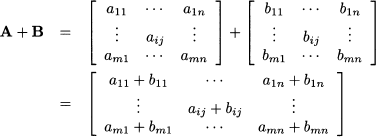
For example

Multiplication by a scalar Given a scalar α , we define its product with a matrix A m,n as follows:

For example

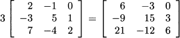
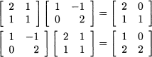
Matrix multiplication We have already seen that elementwise multiplication with vectors does not lead us to an operation with good and interesting properties, whereas the inner product is a rich concept. Matrix multiplication is even trickier, and it is not defined elementwise, either. The matrix product AB is defined only when the number of columns of A and the number of rows of B are the same, i.e., A m,k and B k,n, The result is a matrix, say, C, with m rows and n columns, whose element cij is the inner product of the ith row of A and the jth column of B:

For instance

(3.9)

If two matrices are of compatible dimension, in the sense that they can be multiplied using the rules above, they are said to be conformable. The definition of matrix multiplication does look somewhat odd at first. Still, we may start getting a better felling for it, if we notice how we use it to press a system of linear equations in a very compact form. Consider the system

and group coefficients aij into matrix A n,n, and right-hand sides bi, into column vector b n n,1. Using the definition of matrix multiplication, we may rewrite the system as follows:

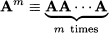
By repeated application of matrix product, we also define the power of a matrix. Squaring a matrix A does not mean squaring each element, but rather multiplying the matrix by itself:

It is easy to see that this definition makes sense only if the number of rows is the same as the number of columns, i.e., if matrix A is a square matrix. By the same token, we may define a generic power:

We may even define the square root of a matrix as a matrix A1/2 such that:

The existence and uniqueness of the square root matrix are not to be taken for granted. We will discuss this further when dealing with multivariate statistics.

A last important observation concerns commutativity. In the scalar case, we know that inverting the order of factors does not change the result of a multiplication: ab = ba. This does not apply to matrices in general. To begin with, when multiplying two rectangular matrices, the number of rows and column may match in such a way that AB is defined, but BA is not. But even in the case of two square matrices, commutativity is not ensured, as the following counterexample shows:

Matrix transposition We have already met transposition as a way of transforming a column vector into a row vector (and vice versa). More generally, matrix transposition entails interchanging rows and columns: Let B = AT be the transposed of A; then bij = aji. For instance

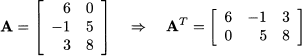
So, if A m,n, then AT n,m.

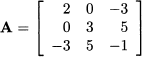
If A is a square matrix, it may happen that A = AT; in such a case we say that A is a symmetric matrix. The following is an example of a symmetric matrix:

Symmetry should not be regarded as a peculiar accident of rather odd matrices; in applications, we often encounter matrices that are symmetric by nature.15 Finally, it may be worth noting that transposition offers another way to denote the inner product of two vectors:

By the same token

The following is an important property concerning transposition and product of matrices.

PROPERTY 3.1 (Transposition of a matrix product) If A and B are conformable matrices, then

We encourage the reader to check the result for the matrices of Eq. (3.9).

Example 3.8 An immediate consequence of the last property is that, for any matrix A, the matrices AT A and AAT are symmetric:

Note that, in general, the matrices AT A and AAT have different dimensions.

3.4.2 The identity matrix and matrix inversion

Matrix inversion is an operation that has no counterpart in the vector case, and it deserves its own section. In the scalar case, when we consider standard multiplication, we observe that there is a “neutral” element for that operation, the number 1. This is a neutral element in the sense that for any x , we have x ˙ 1 = 1 ˙ x = x.

Can we define a neutral element in the case of matrix multiplication? The answer is yes, provided that we confine ourselves to square matrices. If so, it is easy to see that the following identity matrix I n,n will do the trick:

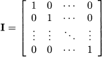
The identity matrix consists of a diagonal of “ones,” and it is easy to see that, for any matrix A n,n, we have AI = IA = A. By the same token, for any vector v n, we have Iv = v (but in this case we cannot commute the two factors in the multiplication).

In the scalar case, given a number x ≠ 0, we define its inverse x-1, such that x ˙ x-1 = x-1 ˙ x = 1. Can we do the same with (square) matrices? Indeed, we can sometimes find the inverse of a square matrix A, denoted by A-1, which is a matrix such that

However, the existence of the inverse matrix is not guaranteed. We will learn in the following text that matrix inversion is strongly related to the possibility of solving a system of linear equations. Indeed, if a matrix A is invertible, solving a system of linear equations like Ax = b is easy. To see this, just premultiply the system by the inverse of A:

Note the analogy with the solution of the linear equation ax = b. We know that x = b/a, but we are in trouble if a = 0. By a similar token, a matrix might not be invertible, which implies that we fail to find a solution to the system of equations. To really understand the issues involved, we need a few theoretical concepts from linear algebra, which we introduce in Section 3.5.

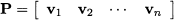
For now, it is useful to reinterpret the solution of a system of linear equations under a different perspective. Imagine “slicing” a matrix A n,n, i.e., think of it as made of its column vectors aj:

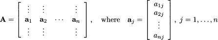
Then, we may see that solving a system of linear equations amounts to expressing the right-hand side b as a linear combination of the columns of A. To illustrate

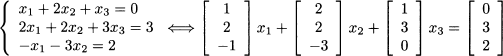
More generally

There is no guarantee that we can always express b as a linear combination of columns aj, j = 1, …, n, with coefficients xj. More so, if we consider a rectangular matrix. For instance, if we have a system of linear equations associated with a matrix in m,n, with m > n, then we have many equations and just a few unknown variables. It stands to reason that in such a circumstance we may fail to solve the system, which means that we may well fail to express a vector with many components, using just a few vectors as building blocks. This kind of interpretation will prove quite helpful later.

3.4.3 Matrices as mappings on vector spaces

Consider a matrix A m,n. When we multiply a vector u n by this matrix, we get a vector v m. This suggests that a matrix is more than just an arrangement of numbers, but it can be regarded as an operator mapping n to m:

Given the rules of matrix algebra, it is easy to see that this mapping is linear, in the sense that:

(3.10)

This means that the mapping of a linear combination is just a linear combination of the mappings. Many transformations of real-world entities are (at least approximately) linear.

If we restrict our attention to a square matrix A n,n, we see that this matrix corresponds to some mapping from n to itself; in other words, it is a way to transform a vector. What is the effect of an operator transforming a vector with n components into another vector in the same space? There are two possible effects:

1. The length (norm) of the vector is changed.

2. The vector is rotated.

In general, a transformation will have both effects, but there may be more specific cases.

If, for some vector v, the matrix A has only the first effect, thus means that, for some scalar λ , we have

A trivial case in which this happens is when A = λI, i.e., the matrix is a diagonal of numbers equal to λ:

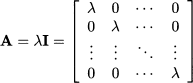
Actually, this is not that interesting, but we will see in Section 3.7 that the condition above may apply for specific scalars (called eigenvalues) and specific vectors (called eigenvectors).

If a matrix has the only effect of rotating a vector, then it does not change the norm of the vector:

This happens if the matrix A has an important property.

DEFINITION 3.2 (Orthogonal matrix) A square matrix P n,n is called an orthogonal matrix if PTP = I. Note that this property also implies that P-1 = PT.

To understand the definition, consider each column vector pj of matrix P. The element in row i, column j of PTP is just the inner product of pi and pj. Hence, the definition above is equivalent to the following requirement:

In other words, the columns of P is a set of orthogonal vectors. To be more precise, we should say orthonormal, as the inner product of a column with itself is 1, but we will not be that rigorous. Now it is not difficult to see that an orthogonal matrix is a rotation matrix. To see why, let us check the norm of the transformed vector y = Pv:

where we have used Property 3.1 for transposition of the product of matrices. Rotation matrices are important in multivariate statistical techniques such as principal component analysis and factor analysis (see Chapter 17).

3.4.4 Laws of matrix algebra

In this section, we summarize a few useful properties of the matrix operations we have introduced. Some have been pointed out along the way; some are trivial to check, and some would require a technical proof that we prefer to avoid.

A few properties of matrix addition and multiplication that are formally identical to properties of addition and multiplication of scalars:

• (A + B) + C = A + (B + C)
• A + B = B + A
• (AB)C = A(BC)
• A(B + C) = AB + AC

Matrix multiplication is a bit peculiar since, in general, AB ≠ BA, as we have already pointed out. Other properties involve matrix transposition:

• (AT)T = A
• (rA)T = rAT
• (A ± B)T = AT ± BT
• (AB)T = BTAT

They are all fairly trivial except for the last one, which we have already pointed out. A few more properties involve inversion. If A and B are square and invertible, as well as of the same dimension, then:

• (A-1)-1 = A
• (AT) = (A-1)T
• AB is invertible and (AB)-1 = B-1A-1

3.5 LINEAR SPACES

In the previous sections, we introduced vectors and matrices and defined an algebra to work on them. Now we try to gain a deeper understanding by taking a more abstract view, introducing linear spaces. To prepare for that, let us emphasize a few relevant concepts:

• Linear combinations. We have defined linear combination of vectors, but in fact we are not constrained to take linear combinations of finite-dimensional objects like tuples of numbers. For instance, we might work with infinite-dimensional spaces of functions. To see a concrete example, consider monomial functions like mk(x) xk. If we take a linear combination of monomials up to degree n, we get a polynomial:

  

  We might represent the polynomial of degree n by the vector of its coefficients:

  

  Note that we are basically expressing the polynomial using “coordinates” in a reference system represented by monomials. However, we could express the very same polynomial using different building blocks. For instance, how can we express the polynomial p(x) = 2 - 3x + 5x2 as a linear combination of e1(x) = 1, e2(x) = 1 - x, and e3(x) = 1 + x + x2? We can ask a similar question with vectors. Given the vector v = [1, 2]T, how can we express it as a linear combination of vectors u1 = [1,0]T and u2 = [1,1]T? More generally, we have seen that solving a system of linear equations entails expressing the right-hand side as a linear combination of the columns of the matrix coefficients. But when are our building blocks enough to represent anything we want? This leads us to consider concepts such as linear independence and the basis of a linear space. We will do so for simple, finite-dimensional spaces, but the concepts that we introduce are much more general and far-reaching. Indeed, if we consider polynomials of degree only up to n, we are dealing with a finite-dimensional space, but this is not the case when dealing with general functions.16

• Linear mappings. We have seen that when we multiply a vector u n by a square matrix A n,n, we get another vector v n, and that matrix multiplication can be considered as a mapping f from the space of n-dimensional vectors to itself: v = f(u) = Au. Moreover, this mapping is linear in the sense of Eq. (3.10). Viewing matrix multiplication in this sense helps in viewing the solution of a system of linear equations as a problem of function inversion. If the image of the linear mapping represented by A is the whole space n, then there must be (at least) one vector x such that b = Ax. Put another way, the set of columns of matrix A should be rich enough to express b as a linear combination of them.
• Linear spaces. Consider the space n of n-dimensional vectors. On that space, we have defined elementary operations such as addition and multiplication by a scalar, which allow us to take linear combinations. If we take an arbitrary combination of vectors in that space, we get another vector in n. By the same token, we see that a linear combination of polynomials of degree not larger than n yields another such polynomial. A linear space is a set equipped with the operations above, which is closed under linear combinations.17

Linear algebra is the study of linear mappings between linear spaces. Before embarking into a study of linear mappings and linear spaces, we consider a motivating example that generalizes the option pricing model of Section 3.1.

3.5.1 Spanning sets and market completeness

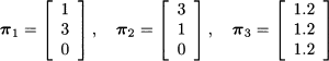
Consider a stylized economy with three possible future states of the world, as illustrated in Fig. 3.9. Say that three securities are available and traded on financial markets, with the following state-contingent payoffs:

Fig. 3.9 A three-state economy: insuring the “bad” state.

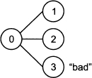
These vectors indicate, e.g., that asset 1 has a payoff 1 if state 1 occurs, a payoff 2 if state 2 occurs, and a payoff 0 in the unfortunate case of state 3. We may notice that the third security is risk-free, whereas state three is bad for the holder of the first and the second security. Let us also assume that the three securities have the following prices now: p1 = p2 = p3 = 1. What should be the price of an insurance against the occurrence of the bad state, i.e., a security paying off 1 if state 3 occurs, and nothing otherwise?

Following the ideas that we have already applied in binomial option pricing, we can try to replicate the payoff of the insurance by a portfolio consisting of an amount αi of each security, for i = 1, 2, 3. Finding the right portfolio requires finding weights such that the payoff vector of the insurance is a linear combination of payoffs πi:

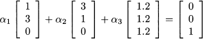
This is just a system of three equations in three unknown variables and yields:

Note that we should sell the two risky securities short. But then, invoking the law of one price, in order to avoid arbitrage opportunities, we may find the fair price of the insurance:

In this case, we are able to price a contingent claim because there is a unique solution to a system of linear equations. In fact, given those three priced assets, we can price by replication any contingent claim, defined on the three future states of the world. In financial economics, it is said that the market is complete.

However, if we enlarge the model of uncertainty to four states, we should not expect to price any contingent claim as we did, using just three “basic” securities. Furthermore, assume that we have three traded securities with the following payoffs:

We immediately see that β3 = β1 + β2. The third security is just a linear combination of the other two and is, in a sense that we will make precise shortly, dependent on them. If we take linear combinations of these three securities, we will not really generate the whole space 3:

We see that, on the basis of these three assets, we cannot generate a security with two different payoffs in states 1 and 2.

Generalizing a bit, when we take a linear combination of vectors and we set weights in any way that we can, we will span a set of vectors; however, the spanned set need not be the whole space n.

3.5.2 Linear independence, dimension, and basis of a linear space

The possibility of expressing a vector as a linear combination of other vectors, or lack thereof, plays a role in many settings. In order to do so, we must ensure that the set of vectors that we want to use as a building blocks is “rich enough.” If we are given a set of vectors v1, v2, …, vm n, and we take linear combinations of them, we generate a linear subspace of vectors. We speak of a subspace, because it is in general a subset of n; it is linear in the sense that any linear combination of vectors included in the subspace belongs to the subspace as well. We say that the set of vectors is a spanning set for the subspace. However, we would like to have a spanning set that is “minimal,” in the sense that all of the vectors are really needed and there is no redundant vector. It should be clear that if one of the vectors in the spanning set is a linear combination of the others, we can get rid of it without changing the spanning set.

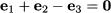
Example 3.9 Consider the unit vectors in 2:

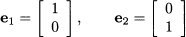
It is easy to see that we may span the whole space 2 by taking linear combinations of e1 and e2. If we also consider vector e3 = [1, 1]T, we get another spanning set, but we do not change the spanned set, as the new vector is redundant:

This can be rewritten as follows:

The previous example motivates the following definition.

DEFINITION 3.3 (Linear dependence) Vectors v1, v2, …, vk n are linearly dependent if and only if there exist scalars α1, α2, …, αk, not all zero, such that

Indeed, vectors e1, e2, and e3 in the example above are linearly dependent. However, vectors e1 and e2 are clearly not redundant, as there is no way to express one of them as a linear combination of the other one.

DEFINITION 3.4 (Linear independence) Vectors v1, v2, …, vk n are linearly independent if and only if

implies α1 = α2 = ˙˙˙ = αk = 0.

Consider now the space n. How many vectors should we include in a spanning set for n? Intuition suggests that

• The spanning set should have at least n vectors.
• If we include more than n vectors in the spanning set, some of them will be redundant.

This motivates the following definition.

DEFINITION 3.5 (Basis of a linear space) Let v1 v2, …, vk be a collection of vectors in a linear space V. These vectors form a basis for V if

1. v1, v2, …, vk span V.

2. v1, v2, …, vk are linearly independent.

Example 3.10 Referring again to Example 3.9, the set {e1, e2, e3} is a spanning set for 2, but it is not a basis. To get a basis, we should get rid of one of those vectors. Note that the basis is not unique, as any of these sets does span 2: {e1, e2}, {e1, e3}, {e2, e3}. These sets have all dimension 2.

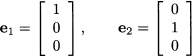
We cannot span 2 with a smaller set, consisting of just one vector. However, let us consider vectors on the line y = x. This line consists of the set of vectors w of the form

This set W is a linear subspace of 2 in the sense that

Vector e3 is one possible basis for subspace W.

The last example suggests that there are many possible bases for a linear space, but they have something in common: They consist of the same number of vectors. In fact, this number is the dimension of the linear space. We also see that a space like n may include a smaller linear subspace, with a basis smaller than n.

As a further example, we may consider the plane xy as a subspace of 3. This plane consists of vectors of the form

and the most natural basis for it consists of vectors

Such unit vectors yield natural bases for many subspaces, but they need not be the only (or the best) choice.

We close this section by observing that if we have a basis, and a vector is represented using that basis, the representation is unique.

3.5.3 Matrix rank

In this section we explore the link between a basis of a linear space and the possibility of finding a unique solution of a system of linear equations Ax = b, where A m,n, x n, and b m. Here, n is the number of variables and m is the number of equations; in most cases, we have m = n, but we may try to generalize a bit.

Recall that our system of equations can be rephrased as

where aj, j = 1, …, n, are the columns of A. We can find a solution only if b is in the linear subspace spanned by the columns of A. Please note that, in order to find a solution, we are not necessarily requiring that the columns of A be linearly independent. This cannot happen if, for instance, we have m = 3 equations and n = 5 variables, because in a space of dimension 3 we cannot find five linearly independent vectors; indeed, the solution need not be unique in such a case. On the other hand, if we have m = 5 equations and n = 3 variables, we will not find a solution in general, unless we are lucky and vector b lies in the subspace (of dimension ≤ 3) spanned by those three columns.

If there is a solution, when is it unique? By now, the reader should not be surprised to learn that this happens when the columns of the matrix are linearly independent, as this imply that there is at most one way to express b using them.

If we consider a square system, i.e., m = n, we are sure to find a unique solution of the system if the columns of the matrix are linearly independent. In such a case, the n columns form a basis for n and we are able to solve the system for any right-hand side b.

Given this discussion, it is no surprise that the number of linearly independent columns of a matrix is an important feature.

DEFINITION 3.6 (Column–row rank of a matrix) Given a matrix A m,n, its column and row ranks are the number of linearly independent columns and the number of linearly independent rows of A, respectively.

A somewhat surprising fact is that the row and the column rank of a matrix are the same. Hence, we may simply speak of the rank of a matrix A m,n, which is denote by rank(A). It is also obvious that rank(A) ≤ min{m, n}. When we have rank(A) = min{m, n}, we say that the matrix A is full-rank. In the case of a square matrix A n,n, the matrix has full rank if there are n linearly independent columns (and rows as well).

Example 3.11 The matrix

is not full rank, as it is easy to check that the third column is a linear combination of the first two columns: a3 = 3a1 + 2a2. Since there are only two linearly independent columns, its rank is 2. The ranks is exactly the same if we look at rows. In fact, the third row can be obtained by adding twice the first row and minus half the second row.

The matrix

has rank 2, since it is easy to see that the rows are linearly independent. We say that this matrix has full row rank, as its rank is the maximum that it could achieve.

We have said that a square system of linear equations Ax = b essentially calls for the expression of the right-hand side vector b as a linear combination of the columns of A. If these n columns are linearly independent, then they are a basis for n and the system can be solved for any vector b. We have also noted that the solution can be expressed in terms of the inverse matrix, x = A-1b, if it exists. Indeed, the following theorem links invertibility and rank of a square matrix.

THEOREM 3.7 A square matrix A n,n is invertible (nonsingular) if and only if rank(A) = n. If the matrix is not full-rank, it is not invertible and is called singular.

The rank of a matrix is a powerful concept, but so far we have not really found a systematic way of evaluating it. Actually, Gaussian elimination would do the trick, but what we really need is a handy way to check whether a square matrix has full rank. The determinant provides us with the answers we need.

3.6 DETERMINANT

The determinant of a square matrix is a function mapping square matrices into real numbers, and it is an important theoretical tool in linear algebra. Actually, it was investigated before the introduction of the matrix concept. In Section 3.2.3 we have seen that determinants can be used to solve systems of linear equations by Cramer’s rule. Another use of the determinant is to check whether a matrix is invertible. However, the use of determinants quickly becomes cumbersome as their calculation involves a number of operations that increases very rapidly with the dimension of the matrix. Hence, the determinant is mainly a conceptual tool.

We may define the determinant inductively as follows, starting from a two-dimensional square matrix:

We already know that for a three-dimensional matrix, we may define the determinant by selecting a row and multiplying its elements by the determinant of the submatrix obtained by eliminating the row and the column containing that element:

(3.11)

The idea can be generalized to an arbitrary square matrix A n as follows:

1. Denote by Aij the matrix obtained by deleting row i and column j of A.

2. The determinant of this matrix, denoted by Mij = det(Aij), is called the (i, j)th minor of matrix A.

3. We also define the (i, j)th cofactor of matrix A as Cij, ( - 1)i+j Mij. We immediately see that a cofactor is just a minor with a sign. The sign is positive if i + j is even; it is negative if i + j is odd.

Armed with these definitions, we have two ways to compute a determinant:

• Expansion by row. Pick any row k, k = 1, …, n, and compute

  

• Expansion by column. Pick any column k, k = 1, …, n, and compute

The process can be executed recursively, and it results ultimately in the calculation of many 2 x 2 determinants. Indeed, for a large matrix, the calculation is quite tedious. The reader is invited to check that Eq. (3.11) is just an expansion along row 1.

3.6.1 Determinant and matrix inversion

From a formal perspective, we may use matrix inversion to solve a system of linear equations:

From a practical viewpoint, this is hardly advisable, as Gaussian elimination entails much less work. To see why, observe that one can find each column aj* of the inverse matrix by solving the following system of linear equations:

Here, vector ej is a vector whose elements are all zero, with a 1 in position j: ej = [0, 0,. 0, 1, 0, …, 0]T. In other words, we should apply Gaussian elimination n times to find the inverse matrix.

There is another way to compute the inverse of a matrix, based on the cofactors we have defined above.

THEOREM 3.8 Let à be a matrix whose element (i, j) is the (j, i)th co-factor Cji of an invertible matrix A: ãij = Cji. Then

The matrix à is called the adjoint of A. In fact, Cramer’s rule (3.6) is a consequence of this theorem. Still, computing the inverse of a matrix is a painful process, and we may see why inverse matrices are not computed explictly quite often. Nevertheless, the inverse matrix is conceptually relevant, and we should wonder if we may characterize invertible matrices in some useful manner.

THEOREM 3.9 A square matrix is invertible (nonsingular) if and only if det(A) ≠ 0.

This should not come as a surprise, considering that when computing an inverse matrix by the adjoint matrix or when solving a system of linear equations by Cramer’s rule, we divide by det(A).

Example 3.12 Using Theorem 3.8, we may prove the validity of a handy rule to invert a 2 x 2 matrix:

In plain terms, to invert a bidimensional matrix, we must

1. Swap the two elements on the diagonal.

2. Change the sign of the other two elements.

3. Divide by the determinant.

3.6.2 Properties of the determinant

The determinant enjoys a lot of useful properties that we list here without any proof.

• For any square matrix A, det(AT) = det(A).
• If two rows (or columns) of A are equal, then det(A) = 0.
• If matrix A has an all-zero row (or column), then det(A) = 0.
• If we multiply the entries of a row (or column) in matrix A by a scalar α to obtain matrix B, then det(B) = α det(A).
• The determinant of a lower triangular, upper triangular, or diagonal matrix is the product of entries on the diagonal.
• The determinant of the product of two conformable matrices A and B is the product of the determinants: det(AB) = det(A) det(B).
• If A is invertible, then det(A-1) = 1/det(A).

3.7 EIGENVALUES AND EIGENVECTORS

In Section 3.4.3 we observed that a square matrix A n,n is a way to represent a linear mapping from the space of n-dimensional vectors to itself. Such a transformation, in general, entails both a rotation and a change of vector length. If the matrix is orthogonal, then the mapping is just a rotation. It may happen, for a specific vector v and a scalar λ, that

Then, if λ > 0 we have just a change in the length of v; if λ < 0 we also have a reflection of the vector. In such a case we say

1. That λ is an eigenvalue of the matrix A

2. That v is an eigenvector of the matrix A

It is easy to see that if v is an eigenvector, then any vector obtained by multiplication by a scalar α , i.e., any vector of form αv, is an eigenvector, too. If we divide a generic eigenvector by its norm, we get a unit eigenvector:

Example 3.13 Consider

(3.12)

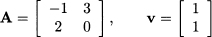
Then we have

Hence, λ = 2 is an eigenvalue of A, and v is a corresponding eigenvector. Actually, any vector of the form [α, α]T is an eigenvector of A corresponding to the eigenvalue λ = 2. The eigenvector

is a unit eigenvector of A.

Matrix eigenvalues are an extremely useful tool with applications in mathematics, statistics, and physics that go well beyond the scope of this book. As far as we are concerned, the following points will be illustrated in this and later chapters:

• Eigenvalues may be used to investigate convexity and concavity of a function.
• They are relevant in optimization applications.
• They are useful in multivariate statistical methods, like principal component analysis, which have a lot of applications, e.g., in marketing and quantitative finance.

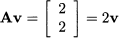
Now we should wonder whether there is a way to compute eigenvalues systematically. In practice, there are powerful numerical methods to do so, but we will stick to the most natural idea, which illustrates a lot of points about eigenvalues. Note that if λ is an eigenvalue and v an eigenvector, we have

(3.13)

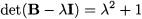
This means that we may express the zero vector by taking a linear combination of the columns of matrix A - λI. A trivial solution of this system is v = 0. But a nontrivial solution can be found if and only if the columns of that matrix are not linearly independent. This, in turn, is equivalent to saying that the determinant is zero. Hence, to find the eigenvalues of a matrix, we should solve the following equation:

(3.14)

This equation is called characteristic equation of the matrix, as eigenvalues capture the essential nature of a matrix.

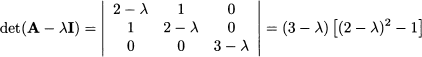
Example 3.14 Let us apply Eq. (3.14) to the matrix A in Eq. (3.12):

This second-order equation has solutions λ1 = 2 and λ2 = -3. These numbers are the eigenvalues of matrix A. To find the eigenvectors corresponding to an eigenvalue, just plug an eigenvalue (say, 2) into the equation (A - λI)v = 0:

These two equations are redundant (the matrix is singular), and by taking either one, we can show that any vector v such that v1 = v2 is a solution of the system, i.e., an eigenvector associated with the eigenvalue λ = 2.

Can we say something about the number of eigenvalues of a matrix? This is not an easy question, but we can say that a n x n matrix can have up to n distinct eigenvalues. To see why, observe that the characteristic equation involves a polynomial of degree n, which may have up to n distinct roots. In general, we can state what follows:

• Eigenvalues may be complex conjugates, rather than real numbers; for instance, consider the following matrix:

  

  The characteristic polynomial is

  

  Hence, the two eigenvalues are λ = ±i, where i is the unit imaginary number defined by i2 = -1. We do not find real eigenvalues, but this is not surprising as matrix B is a matrix rotating a vector by π/2, i.e., 90° on the plane. (Please check this graphically!)

• Eigenvalues may be multiple roots of the characteristic polynomial, as in the case λ2 + 2λ + 1 = (λ + 1)2 = 0. When there are multiple eigenvalues, finding eigenvalues may be tricky, but we can do without these technicalities.

The following properties of the eigenvalues of a matrix A are worth mentioning here:

• The determinant of the matrix is the product of the eigenvalues: det(A) .
• The trace of the matrix, which is just the sum of its entries on the diagonal, is the sum of the eigenvalues: .

The first property has an interesting consequence: The matrix A is singular (hence, not invertible) when one of its eigenvalues is zero.

3.7.1 Eigenvalues and eigenvectors of a symmetric matrix

In applications, it is often the case that the matrix A is symmetric.18 A symmetric matrix has an important property.

THEOREM 3.10 Let A n be a symmetric matrix. Then

1. The matrix has only real eigenvalues.

2. The eigenvectors are mutually orthogonal.

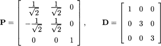
The second point in the theorem implies that if we form a matrix P using normalized (unit) eigenvectors

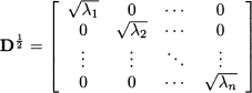
this matrix is orthogonal, i.e., PTP = I and P-1 = PT. This allows us to build a very useful factorization of a symmetric matrix A:

If we denote by D the diagonal matrix consisting of the n eigenvalues, we see that we may factor matrix A as follows:

(3.15)

Going the other way around, we may “diagonalize” matrix A as follows:

(3.16)

Example 3.15 Consider the following matrix:

Its characteristic polynomial can be obtained by developing the determinant along the last row:

We immediately see that its roots are

They are three real eigenvalues, as expected, but one is a multiple eigenvalue. To find the eigenvectors, let us plug λ = 3 into Eq. (3.13):

From the last row of the matrix, we see that v3 can be chosen freely. Furthermore, we see that the first and the second equation are not linearly independent. In fact, the rank of matrix A is 1, and we may find two linearly independent eigenvectors of the form

Let us choose

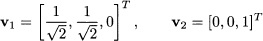
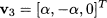
in order to have two orthogonal and unit eigenvectors. We leave as an exercise for the reader to verify that, if we plug the eigenvalue λ = 1, we obtain eigenvectors of the form

Now, we may check that

where

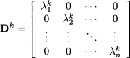
Luckily, there are efficient and robust numerical methods for finding eigenvalues and eigenvectors, as well as for diagonalizing a matrix. These methods are implemented by widely available software tools. What is more relevant to us is the remarkable number of ways in which we may take advantage of the results above. As an example, the computation of powers of a symmetric matrix, Ak, is considerably simplified:

where

By the same token, we may compute the square root of a matrix, i.e., a matrix A1/2 such that A = A1/2A1/2

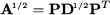
where

Matrix inversion is easy, too:

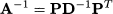
where D-1 = diag(λ1-1, λ2-1, …, λn-1,). Here we have used a shorthand notation to denote a diagonal matrix by just giving its diagonal elements.

3.8 QUADRATIC FORMS

In the last two sections of this chapter, we explore the connections between linear algebra and calculus. This is necessary in order to generalize calculus concepts to functions of several variables; since any interesting management problem involves multiple dimensions, this is a worthy task. The simplest nonlinear function of multiple variables is arguably a quadratic form:

(3.17)

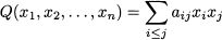
Denoting the double sum as is typically preferred to , as the latter is a bit ambiguous. To see the issue, consider a term such as 4x1x2; we could rewrite this as 3x1x2 + x2x1 or 2x1x2 + 2x2x1. The notation above results in a unique way of expressing a quadratic form. Concrete examples of quadratic forms are

(3.18)

Quadratic forms are important for several reasons:

1. They play a role in the approximation of multivariable functions using Taylor expansions; in Section 3.9 we will see how we can generalize the Taylor expansion of Section 2.10.

2. Quadratic forms are also important in nonlinear optimization (see Section 12.5).

3. In probability and statistics, the variance of a linear combination of random variables is linked to a quadratic form (Section 8.3); this is fundamental, among many other things, in financial portfolio management.

Quadratic forms are strongly linked to linear algebra as they can be most conveniently associated with a symmetric matrix. In fact, we may also express any quadratic form as

(3.19)

where matrix A is symmetric. For instance, we can express the quadratic forms in Eq. (3.18) as follows:

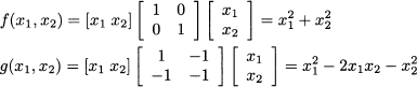
Note that cross-product terms correspond to off-diagonal entries in the matrix; in fact, the aij coefficients in expression (3.17), for i ≠ j, occur divided by 2 in the matrix. These two quadratic forms are plotted in Figs. 3.10 and 3.11, respectively. From what we know about convexity (Section 2.11), we immediately see that f is convex, whereas g is neither convex nor concave, as it features a “saddle point.” Convexity and concavity of a quadratic form are linked to properties of the corresponding matrix.

Fig. 3.10 A convex quadratic form.

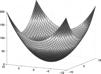
Fig. 3.11 An undefined quadratic form.

DEFINITION 3.11 (Definiteness of quadratic forms) We say that a quadratic form xT Ax

• Is positive definite if xT Ax > 0 for all x ≠ 0
• Is positive semidefinite if xT Ax ≥ 0 for all x
• Is negative definite if xT Ax < 0 for all x ≠ 0
• Is negative semidefinite if xT Ax ≤ 0 for all x

Otherwise, we say that the quadratic form is indefinite.

The definiteness of a quadratic form is strictly related to convexity by the following properties:

• A positive definite quadratic form is a strictly convex function.
• A positive semidefinite quadratic form is a convex function.
• A negative definite quadratic form is a strictly concave function.
• A negative semidefinite quadratic form is a concave function.

Incidentally, we may observe that for a positive definite quadratic form, the origin x* = 0 is a global minimizer, as it is the only point at which the function is zero, whereas it is strictly positive for any x ≠ 0. By the same token, x* = 0 is a global maximizer for a negative definite quadratic form. For semidefinite forms, there may be alternative optima, i.e., several vectors x for which the function is zero.

Now the main problem is to find a way to check the definiteness of a quadratic form. A good starting point is to observe that this task is easy to accomplish for a diagonal matrix:

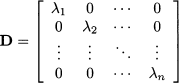
In such a case, the quadratic form does not include cross-products:

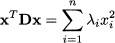
It is easy to see that definiteness of this quadratic form depends on the signs of the diagonal terms λi. If they are all strictly positive (negative), the form is positive (negative) definite. If they are nonnegative (nonpositive), the form is positive (negative) semidefinite. But for a diagonal matrix, the entries on the diagonal are just its eigenvalues. Since the matrix associated with a quadratic form is symmetric, we also know that all of its eigenvalues are real numbers. Can we generalize and guess that definiteness depends on the sign of the eigenvalues of the corresponding symmetric matrix? Indeed, this is easily verified by factorizing the quadratic form using Eq. (3.15)

where y = PTx. This is just another quadratic form, which has been diagonalized by a proper change of variables. We may immediately conclude that a quadratic form

• Is positive definite if and only if the eigenvalues of the corresponding matrix A are all strictly positive (> 0)
• Is positive semidefinite if and only if the eigenvalues of the corresponding matrix A are all nonnegative (≥ 0)
• Is negative definite if and only if the eigenvalues of the corresponding matrix A are all strictly negative (< 0)
• Is negative semidefinite, if and only if the eigenvalues of the corresponding matrix A are all nonpositive (≤ 0)

3.9 CALCULUS IN MULTIPLE DIMENSIONS

In this section we extend some concepts that we introduced in the previous chapter, concerning calculus for functions of one variable. What we really need for what follows is to get an intuitive idea of how some basic concepts are generalized when we consider a function of multiple variables, i.e., a function f(x1, x2, …, xn) = f(x) mapping a vector in n to a real number. In particular, we would like to see

1. How we can extend the concept of derivative

2. How we can extend the Taylor’s expansion

3. What is an integral in multiple dimensions

The first two issues are relevant from an optimization perspective, and they are strictly linked to linear algebra. Multiple integrals play a more limited role in the book, as they will be used only to deal with probability distributions of multiple random variables.

3.9.1 Partial derivatives: gradient and Hessian matrix

In Section 2.7 we defined the derivative of a function of a single variable as the limit of an increment ratio:

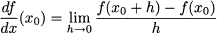
If we have a function of several variables, we may readily extend the concept above by considering a point x0 = [x10, …, xn0]T and perturbing one variable at a time. We obtain the concept of a partial derivative with respect to a single variable xi.

As in the single-variable case, we should not take for granted that the limit above exists, but we will not consider too many technicalities. In practice, the limit above is readily computed by applying the usual rules for derivatives, considering one variable at a time and keeping the other variables fixed. For a function of n variables, we have n (first-order) partial derivatives at a point x0. They can be grouped into a column vector in n, which is called the gradient of f at point x0:

Example 3.16 Consider the quadratic form f(x1, x2) = x12 + x22. We may compute the following partial derivatives:

When computing the partial derivative with respect to x1, we consider x2 as a constant, and this explains why x2 does not contribute to the first partial derivative. The two partial derivatives can be grouped into the gradient

To see a more contrived example, consider the following function:

We invite the reader to verify that its gradient is

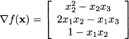
How can we interpret the gradient? We know from single variable calculus that a stationary point is a natural candidate to be a minimum or a maximum of a function; at that point, the tangent line is horizontal. In the multivariable case, we can say something similar by referring to the gradient. A stationary point (or point of stationarity) is a point x* such that the gradient is the zero vector: f(x*) = 0. For instance, the origin is a stationary point of the quadratic form in the example above. Geometric interpretation is difficult for several variables, but in the case of two variables, the function is graphed in three dimensions and a stationary point is characterized by a horizontal tangent plane. In general, it can be shown that the gradient is a vector pointing toward the direction of maximum ascent of the function.

Example 3.17 Consider again the quadratic form x12 + x22, and its gradient. The function is just the squared distance of each point from the origin and its level curves are concentric circles, as shown in Fig. 3.12. The figure also shows the gradient vector for a few points on a level curves. We see that the gradient f(x1, x2) at each point is a vector moving away from the origin toward infinity, and along that direction the function has the steepest ascent. If we change the sign of the gradient, we get a vector pointing toward the origin, and spotting the path of steepest descent.

Fig. 3.12 The gradient gives the direction of maximum ascent at each point.

It is easy to understand that this feature of the gradient is relevant to function maximization and minimization.

The gradient vector collects the first-order partial derivatives of a function with respect to all of the independent variables. We may also consider second-order derivatives by repeated application of partial differentiation. If we take a derivative of function f twice with respect to the same variable xi, we have the second-order partial derivative, which is denoted as

We may also take the derivative with respect to two different variables, which yields a mixed derivative; if we take partial derivative first with respect to xi, and then with respect to xj, we obtain

An immediate question is if the order with which derivatives are taken is relevant or not. The answer is that, when suitable continuity conditions are met, the order in which we take derivatives is inconsequential:19

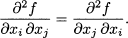
If we group second-order partial derivatives into a matrix, we obtain the Hessian matrix:

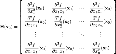
Since the order of variables in mixed terms is not relevant, the Hessian matrix is symmetric.

Example 3.18 Let us find the Hessian matrix for the quadratic forms:

First, we calculate all of the relevant partial derivatives for f:

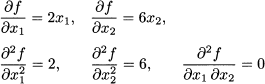
The Hessian matrix of f is diagonal:

The reader is invited to verify that, in the case of g, we obtain

From the example, we immediately notice that this Hessian matrix is just twice the matrix associated with the quadratic form. Indeed, if we write a quadratic form as

(3.20)

we see that matrix A is its Hessian. Another useful result concerning quadratic forms written in the form of Eq. (3.20) is

(3.21)

The result is easy to check directly.

3.9.2 Taylor’s expansion for multivariable functions

Using the gradient and Hessian matrix, we may generalize Taylor’s expansion to functions of multiple variables. The second-order expansion around point x0 is as follows:

We see that this approximation boils down to Eq. (2.13) when considering a function of a single variable. If we stop the expansion to first-order terms, we get a linear approximation, which is just a plane when working with functions of two variables. Such a tangent plane is illustrated in Fig. 3.13. The inclusion of the second-order terms implies that the approximation involves a quadratic form. The approximation can be convex, concave, or neither, depending on the definiteness of the quadratic form corresponding to the Hessian matrix. Hence, the eigenvalues of the Hessian matrix are useful in analyzing convexity/concavity issues and in checking optimality conditions.

Fig. 3.13 First-order Taylor expansion yields a tangent plane.

Example 3.19 Let us compute Taylor’s expansion of function

in a neighborhood of point (1, 1). The partial derivatives are

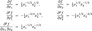
Evaluating gradient and Hessian at (1, 1) yields

Note that, unlike a quadratic form, Taylor’s expansion of f depend on the point at which it is taken. Considering small displacements δ1 and δ2 around x1 = 1 and x2, we get

The eigenvalues of the Hessian matrix are λ1 = -0.5 and λ2 = 0. One of the eigenvalues is zero, and indeed it is easy to see that the Hessian matrix is singular. Moreover, the eigenvalues are both nonpositive, suggesting that the function f is locally concave, but not strictly. A surface plot of the function is illustrated in Fig. 3.14, for positive values of x1 and x2; from the figure, we see the concavity of the function in this region. A closer look at the surface explains why the function is not strictly concave there. For x1 = x2, we have . Hence, the function is linear along that direction.

Fig. 3.14 Surface plot of function x1x2.

3.9.3 Integrals in multiple dimensions

Definite integrals have been introduced in Section 2.13 as a way to compute the area below the curve corresponding to the graph of a function of one variable. If we consider a function (x, y) of two variables, there is no reason why we should not consider its surface plot and the volume below the surface, corresponding to a region D on the (x, y) plane. This double integral is denoted as follows:

and the idea is illustrated in Fig. 3.15. Here, the domain on which the function is integrated is a rectangle, but more general shapes are allowed. Nevertheless, rectangular tiles are easy to deal with, and indeed they are the basis for a rigorous definition of the double integral. In the following chapters, we will encounter double integrals only when characterizing the joint distribution of two random variables, in Section 8.1, and we just need an intuitive understanding.

Fig. 3.15 Double integral as a volume below a surface graph of a function.

To compute a double integral, a convenient way is to regard double integrals as iterated integrals, over a rectangular domain [a, b] x [c, d]:

Please note the order of differentials dy and dx: Here we want to point out the ordering of variables with which the integration is carried out. If we want to be precise, we could write

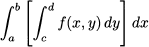
The idea behind iterated integration is straightforward: We should first integrate with respect to y, treating x as a constant, obtaining a function of x that is then integrated with respect to x.

Example 3.20 Consider function f(x, y) = x2y and the rectangular domain [1,2] x [-3, 4] obtained by taking the Cartesian product of intervals [1, 2] on the x-axis and [-3, 4] on the y-axis. We want to find the following integral:

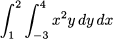
In the inner integral, x can be regarded as a constant and, in this case, it can be just taken outside:

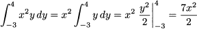
Then, we proceed with the outer integral:

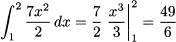
The conditions under which a double integral can be tackled as an iterated integral are stated by Fubini’s theorem, and the idea can be generalized to multiple dimensions.

Problems

3.1 Solve the system of linear equations:

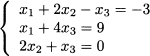
using both Gaussian elimination and Cramer’s rule.

3.2 Express the derivative of polynomials as a linear mapping using a matrix.

3.3 Prove that the representation of a vector using a basis is unique.

3.4 Let A m,n, and let D be a diagonal matrix in n,n. Prove that the product AD is obtained by multiplying each element in a row of A by the corresponding element in the diagonal of D. Check with

3.5 Unlike usual algebra, in matrix algebra we may have AX = BX, even though A ≠ B and X ≠ 0. Check with

3.6 Consider the matrix H = I -hhT, where h is a column vector in n and I is the properly sized identity matrix. Prove that H is orthogonal, provided that hTh = 1. This matrix is known as the Householder matrix.

3.7 Consider the matrix C = In - 1/n Jn, where In n,n is the identity matrix and Jn n,n is a matrix consisting of 1. This matrix is called a centering matrix, since xTC = {xi - $xB}, where x = [x1,x2, …, xn] is a vector of observations. Prove this fact. Also prove that

3.8 Check that the determinant of diagonal and triangular matrices is the product of elements on the diagonal.

3.9 Find the inverse of each of the following matrices

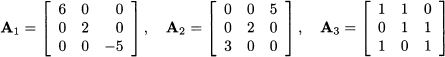
3.10 For a square matrix A, suppose that there is a vector x ≠ 0 such that Ax = 0. Prove that A is singular.

3.11 Prove that hhT - hThI is singular.

3.12 Prove that two orthogonal vectors are linearly independent.

3.13 Show that if λ is an eigenvalue of A, then 1/(1 + λ) is an eigenvalue of (I + A)-1.

3.14 Show that, if the eigenvalues of A are positive, those of A + A-1 are not less than 2.

3.15 Prove that, for a symmetric matrix A, we have

where λk, k = 1, …, n, are the eigenvalues of A.

For further reading

• A short and readable introduction to linear algebra can be found, e.g., in the text by Lang [4].
• A more advanced treatment, paying some more attention to matrix analysis, is offered by Meyer [6]
• Since the actual reason why we are interested in matrix algebra is its role in multivariate statistics, the reader might be interested in references which are specifically aimed at this kind of application, such as Refs. [2] or [7]; a few exercises have been taken from the latter reference.
• A good reference for multivariable calculus is Ref. [5]. Since this excellent reference takes a quite general perspective, including some concepts that are more relevant in physics, the reader might wish to consult a more economically oriented reference: Ref. [8] covers single- and multi-variable calculus, as well as linear algebra and matrix analysis.
• We have opened this chapter mentioning option pricing. The standard reference for financial derivatives is the book by Hull [3]; a text that is more focused on computational methods in finance is Ref. [1].

REFERENCES

1. P. Brandimarte, Numerical Methods in Finance and Economics: A Matlab-Based Introduction, 2nd ed., Wiley, New York, 2006.

2. D.H. Harville, Matrix Algebra from a Statistician’s Perspective, Springer, New York, 1997.

3. J.C. Hull, Options, Futures, and Other Derivatives, 5th ed., Prentice Hall, Upper Saddle River, NJ, 2003.

4. S. Lang, Introduction to Linear Algebra, 2nd ed., Springer, New York, 1986.

5. S. Lang, Calculus of Several Variables, 3rd ed., Springer, New York, 1987.

6. C.D. Meyer, Matrix Analysis and Applied Linear Algebra, Society for Industrial and Applied Mathematics, Philadelphia, 2000.

7. S.R. Searle, Matrix Algebra Useful for Statistics, Wiley, New York, 1982.

8. C.P. Simon and L. Blume, Mathematics for Economists, W.W. Norton, New York, 1994.

1 See Chapter 17.

2 We assume that the option can only be exercised at maturity. Such an option is called European-style. On the contrary, American-style options can be exercised at any time before their expiration date.

3 The binomial model is basically related to coin flipping; see Section 1.2.3.

4 An arbitrage opportunity is essentially a riskless money-making machine exploiting price inconsistencies. We have considered arbitrage opportunities when discussing a forward contract in Section 1.3.1.

5 See Section 2.3.4 for an introduction to continuous compounding.

6 The result is easily obtained by applying Cramer’s rule of Section 3.2.3.

7 See Example 1.3 for an illustration of short selling.

8 The concept of expected value E[X] of a random variable will be fully treated later. For now, you may safely assume that it is equivalent to the intuitive concept of mean, using probabilities of future events rather than relative frequencies resulting from the observation of past data.

9 The careful reader should wonder if we can take advantage of the element a33 = 0 in the matrix by developing the determinant along the last row, rather than along the first one; indeed, this can be done by the rules illustrated in Section 3.6.

10 In physics, there is another definition of vector product, which is not useful in our setting.

11 Indeed, the inner product is sometimes referred to as the “scalar product.” We will avoid this term, as it may be confused with multiplication by a scalar.

12 Later, we will learn that two random variables are “orthogonal” if they are uncorrelated.

13 For instance, Euclidean norm is used in standard linear regression by least squares; see Section 10.1.1 for alternative approaches.

14 The reader might appreciate the definition of convex combination a little better by referring back to Section 2.11 on convexity. We will also see that coefficients with those properties might be interpreted as probabilities, as they are nonnegative and add up to one; hence, a convex combination bears some resemblance to the probabilistic concept of expected value.

15 One such common example that we will meet later is the matrix collecting all of the covariances between a vector of random variables.

16 To see this, consider the Taylor expansion of Section 2.10; to approximate a continuous function to an arbitrary accuracy, we should let the degree of the polynomial go to infinity.

17 A rigorous definition involves a much longer listing of properties (see, e.g., Ref. [4]), but we will just settle for the basic idea.

18 In probability and statistics, we use covariance matrices, which are symmetric; see Section 8.3. In optimization, symmetric matrices are used to define a quadratic form; see Section 3.9 on multidimensional calculus.

19 This result is known as Young’s theorem.