Chapter 15
Introduction to Multivariate Analysis
Multivariate analysis is the more-or-less natural extension of elementary inferential statistics to the case of multidimensional data. The first difficulty we encounter is the representation of data. How can we visualize data in multiple dimensions, on the basis of our limited ability to plot bidimensional and tridimensional diagrams? In Section 15.1 we show that this is just one of the many issues that we may have to face. The richness of problems and applications of multivariate analysis has given rise to a correspondingly rich array of methods. In the next two chapters we will outline a few of them, but in Section 15.2 we offer a more general classification. Finally, the mathematics involved in multivariate analysis is certainly not easier than that involved in univariate inferential statistics. Also probability theory in the multidimensional case is more challenging than what we have seen in the first part of the book, and the limited tools of correlation analysis should be expanded. However, for the limited purposes of the following treatment, we just need a few additional concepts; in Section 15.3 we illustrate the important role of linear algebra and matrix theory in multivariate methods.
15.1 ISSUES IN MULTIVARIATE ANALYSIS
In the next sections we briefly outline the main complication factors that arise when dealing with multidimensional data. Some of them are to be expected, but some are a bit surprising. Getting aware of these difficulties provides the motivation for studying the wide array of sometimes quite complex methods that have been developed.
15.1.1 Visualization
The first and most obvious difficulty we face with multivariate data is visualization. If we want to explore the association between variables, one possibility is to draw scatterplots for each pair of them; for instance, if we have 4 variables, we may draw a matrix of scatterplots, like the one illustrated in Fig. 15.1. The matrix of plots is symmetric, and the histograms of each single variable are displayed on the diagonal. Clearly, this is a rather partial view, even though it can help in spotting pairwise relationships. Many fancy methods have been proposed to obtain a more complete picture of multivariate data, such as drawing human faces, whose features are related to data characteristics; however, they may be rather hard to interpret. A less trivial approach is based on data reduction. Quite often, even though there are many variables, we may take linear combinations of them in such a way that a limited number of such transformations includes most of the really interesting information. Such an approach is principal component analysis, which is illustrated in Chapter 17.
Fig. 15.1 A matrix of scatterplots.

15.1.2 Complexity and redundancy
Visualization is not the only reason why we need data reduction methods. Quite often, multivariate data stem from the administration of a questionnaire to a sample of respondents; each question corresponds to a single variable, and a set of answers by a single respondent is a multivariate observation. It is customary to ask respondents many related questions, possibly in order to check the coherence in their answers. However, an unpleasing consequence is that some variables may be strictly related, if not redundant. On the one hand, this motivates the use of data reduction methods further. On the other hand, this may complicate the application of rather standard approaches, such as multiple linear regression. In Chapter 16, we will see that a strong correlation between variables may result in unreliable regressed models; this issue is known as collinearity. By reducing the number of explanatory variables in the regression model, we may ease collinearity issues. Another common issue is that when a problem has multiple dimensions, it is difficult to group similar observations together. For instance, a common task in marketing is customer segmentation. In Chapter 17 we also outline clustering methods that may be used to this aim.
15.1.3 Different types of variables
In standard inferential statistics one typically assumes that data consist of real or integer numbers. However, data may be qualitative as well, and the more dimensions we have, the more likely the joint presence of quantitative and qualitative variables will be. In some cases, dealing with qualitative variables is not that difficult. For instance, if we are building a multiple regression model that includes one or more qualitative explanatory variables, we may represent them as binary (dummy) variables, where 0 and 1 correspond to “false” and “true,” respectively. However, things are not that easy if it is the regressed variable that is binary. For instance, we might wish to estimate the probability of an event on the basis of explanatory variables; this occurs when we are evaluating the creditworthiness of a potential borrower, on the basis of a set of personal characteristics, and the output is the probability of default. Another standard example is a marketing model to predict purchasing decisions on the basis of product features. Adapting linear regression to this case calls for less obvious transformations, leading to logistic regression, which is also considered in Chapter 16. In other cases, the qualitative nature of data calls for methods that are quite different from those used for quantitative variables.
15.1.4 Adapting statistical inference procedures
The core topics in statistical inference are point and interval parameter estimation, hypothesis testing, and analysis of variance. Some of the related procedures are conceptually easy to adapt to a multivariate case. For instance, maximum likelihood estimation is not quite different, even though it is going to prove computationally more challenging, thus requiring numerical optimization methods for the maximization of the likelihood function. In other cases, things are not that easy and may call for the introduction of new classes of multivariable probability distributions to characterize data. The following example shows that a straightforward extension of single-variable (univariate) methods may not be appropriate.
Example 15.1 Let us consider a hypothesis test concerning the mean of a multivariate probability distribution. We want to check the hypothesis that the expected value of a jointly normal random variable  . Therefore, we test the null hypothesis

against the alternative one

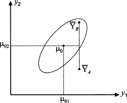
The random vector Y has components Y1 and Y2; let us denote the two components of vector μ0 by μ01 and μ02, respectively. One possible approach would be to calculate the sample mean of each component,  1 and 2, and run two univariate tests, one for μ01 and one for μ02. More precisely, we could test the null hypothesis H0: μ1 = μ01 on the basis of the sample mean 1, and H0: μ2 = μ02 on the basis of the sample mean 2. Then, if we reject even one of the two null univariate hypotheses, we reject the multivariate hypothesis as well. Unfortunately, this approach may fail, as illustrated in Fig. 15.2. In the figure, we show an ellipse, which is a level curve of the joint PDF, and two possible sample means, corresponding to vectors A and B. The rotation of the ellipse corresponds to a positive correlation between Y1 and Y2. If we account for the nature of the PDF of jointly normal variables (see Section 8.4), it turns out that the acceptance region for the test above should be an’ ellipse. Let us assume that the ellipse in Fig. 15.2 is the acceptance region for the test; then, in the case of A, the null hypothesis should be rejected; in the case of B, we do not reject H0. On the contrary, testing the two hypotheses separately results in a rectangular acceptance region around μ0 (the rectangle is a square if the two standard deviations are the same). We immediately observe that, along each dimension, the distance between μ0 and A and the distance between μ0 and B are exactly the same, in absolute value. Hence, if we run separate tests, we either reject or accept the null hypothesis for both sample means, which is not correct. The point is that a rectangular acceptance region, unlike the elliptical one in Fig. 15.2, does not account for correlation.
Fig. 15.2 A bidimensional hypothesis test.
Incidentally, a proper analysis of the testing problem in Example 15.1 leads to consider the test statistic

where S-1 is the inverse of the sample covariance matrix. Hence, distributional results for univariate statistics, which involve a t distribution, must be extended by the introduction of a new class of probability distributions, namely, Hotelling’s T2 distribution.
15.1.5 Missing data and outliers
Outliers and wrong data are quite common in data analysis. If data are collected automatically, and they are engineering measurements, this may not be a tough issue; however, when people are involved, either because we are collecting data using questionnaires, or because we are investigating a social system, things may turn out to be a nightmare. Having to cope with multidimensional data will naturally exacerbate the issue. While an outlier may be easy to “see” in one-dimensional data, possibly using a boxplot,1 it is not obvious at all how an outlier is to be spotted in 10 or more dimensions. Again, data reduction techniques may help. Missing data may also be the consequence of real or perceived redundancy. The following example illustrates a counterintuitive effect.
Example 15.2 Imagine collecting data in a city logistics problem. One of the most important measures is the percentage saturation of vehicles. No one would like the idea of half-empty vehicles polluting air more than necessary in congested urban traffic. So, one would naturally want to investigate the real level of vehicle saturation to check whether some improvement can be attained by proper reorganization. However, capacity is multidimensional. Probably, the most natural capacity measure that comes to mind is volume capacity.2 However, weight may be the main issue with certain types of items; before dismissing this issue, think of the impact of weight on the space needed to brake a fully loaded truck. Moreover, if small parcels are delivered, the binding
Table 15.1 Difficulties with missing multidimensional data.
constraint on a vehicle tour will be neither volume nor weight, but time, since driving shifts are constrained.
Now, imagine administering a questionnaire to truck drivers, asking them an estimate of their average saturation level, in percentage, with respect to the three dimensions of capacity. The result might look like the fictional data in Table 15.1. There, we show the hypothetical result of three interviews. The first truck driver answered that he is 100% saturated in terms of time; the binding factor here is the number of deliveries, and he did not provide any answer in terms of the other two capacity dimensions, as they are not relevant to him and he had no clue. The second driver was quite thorough, whereas the third one did not consider time. In the table, we also give the maximum saturation percentage in the last column, over the three capacity dimensions, for each driver. The last row gives the average over drivers, for each dimension. Finally, we also consider the average of the maximum saturation for each driver. Do you see something wrong here?
The average of the maxima is
but if we take the average saturation with respect to time, we get a larger number:
This should not be the case, however: How can the average of maxima across dimensions (68.33%) be less than the average with respect to one dimension (70%)? This surprising fact is, of course, the result of missing data.
The example above may look somewhat pathological, since very few data are displayed; on the contrary, this is what happened in a real-life case, and we display fictional data in Table 15.1 just to illustrate the issue more clearly.3
The higher the number of dimensions, the more severe the issues with missing data will be. The hard way to solve this issue is to discard incomplete data, but this may considerably reduce the sample. Another strategy is to fill the holes by using regression models. We may fit regression models with available data, and we compute the missing pieces of information as a function of what is available. Clearly, this does sound a bit arbitrary, but it may be better than ending up with a very small and useless set of complete data.
15.2 AN OVERVIEW OF MULTIVARIATE METHODS
Multivariate methods can be classified along different features:
- Confirmatory vs. exploratory. This feature refers to the general aim of a method, as some are aimed at confirming a theory or a hypothesis, and others are aimed at analyzing data and discovering hidden patterns.
- Metric vs. nonmetric. This feature refers to the kind of variables that the method is able to deal with, i.e., quantitative or qualitative. We recall that sometimes numerical codes are associated with qualitative variables, which have no real content. In such a case, we speak of nominal scales.4 When variables are quantitative, we distinguish the following types of scale:
— Ordinal scales, where variables have numerical values that can sensibly ordered, but their differences have no meaning. As an example, imagine a set of customers ranking different brands by assigning a numerical evaluation.
— Interval scales, where differences between numerical values have a meaning, but there is no “natural” origin of the scale. For instance, consider temperatures, which can be measured with different scales.
— Ratio scales, where there is an objective reference point acting as the origin of the scale.
- Interdependence vs. dependence. When we are focusing on dependence, there is a clear separation between the set of independent variables (e.g., factors) and the set of dependent variables (e.g., effects). One such case is simple linear regression. In interdependence analysis there is no such clear-cut distinction.
In the following sections we outline some multivariate methods, suggesting a classification along the above dimensions. We do not aim at being comprehensive; the idea is getting to appreciate the richness of this field of statistics, as well as the classification above in concrete terms.
15.2.1 Multiple regression models
In regression models there is a clear separation between the regressed variable and the regressors (explanatory variables):

This does not necessarily mean that there is a causal relationship, but it is enough to classify regression models as dependence models. Regression models arise naturally for dealing with metric variables, but we may use binary variables to model qualitative features in a limited way. We may use regression models for confirming a theory, by testing the significance of individual coefficients or the overall significance of the whole model, as we show in Chapter 16. However, we may also use the technology as an exploratory tool, by running a sequence of regression models involving different sets of regressors. Furthermore, logistic regression models allow for a qualitative regressed variable taking only two values. Alternative methods, such as discrete discriminant analysis, may be used for the case of a dependent categorical variable assuming more than two values.
15.2.2 Principal component analysis
Principal component analysis (PCA) is a data reduction method. Technically, we take a vector of random variables X 
 m, and we transform it to another vector Z m, by a linear transformation represented by a square matrix A m,m. In more detail we have
These equations should not be confused with regression equations. The transformed Zi variables are not observed and used in a fitting procedure; indeed, there is no error term. They are just transformations of the original variables, which are not classified as dependent or independent. Hence, PCA is an interdependence technique, aimed at metric data, and used for exploratory purposes. In Section 17.2 we show that, by taking suitable combinations, we may find a small subset of Zi variables, the principal components, that explain most of the variability in the original variables Xi. By disregarding the less relevant components, we reduce data dimensionality without losing a significant portion of information.
15.2.3 Factor analysis
Factor analysis is another interdependence technique, which shares some theoretical background with PCA, as we show in Section 17.3. Factor analysis can be used for data reduction, too, but it should not be confused with PCA, as in factor analysis we are looking for hidden factors that may explain common sources of variance between variables. Formally, we aim at finding a model such as
where the variables Yi are what we observe, Fj are common underlying factors, i are individual sources of variability, and m is significantly smaller than p. This may look like a set of regression models, but the main difference is that factors are not directly observable. We are trying to uncover hidden factors, which have to be interpreted. Even though the above equations suggest a dependence structure between the observations and the underlying factors, there is no dependence structure among the observations themselves; hence, factor analysis is considered an interdependence method for dealing with metric data. It is natural to use factor analysis for exploratory purposes, but it can also be used for confirmatory purposes.
15.2.4 Cluster analysis
The aim of cluster analysis is categorization, i.e., the creation of groups of objects according to their similarities. The idea is hinted at in Fig. 15.3. There are other methods, such as discriminant analysis, essentially aimed at separating groups of observations. However, they differ in the underlying-approach, and some can only deal with metric data. Cluster analysis relies on a distance measure; hence, provided we are able to define a distance with respect to qualitative attributes, it can cope with nonmetric variables. There is an array of cluster analysis methods, which are exploratory and aimed at studying interdependence; they are outlined in Section 17.4.
Fig. 15.3 Four bidimensional clusters.

15.2.5 Canonical correlation
Consider two sets of variables that are collected in vectors X and Y, respectively, and imagine that we would like to study the relationship between the two sets. One way for doing so is by forming two linear combinations, Z = aTX and W = bTY, in such a way that the correlation ρZ,W is maximized. This is what is accomplished by canonical correlation, or canonical analysis. Essentially, the idea is to study the relationship between groups of metric variables by relating low-dimensional projections. When Y reduces to a scalar random variable Y, canonical correlation boils down to multiple linear regression. To illustrate one potential application of canonical correlation, consider a set of marketing activities (advertising effort, packaging quality and appeal, pricing, bundling of products and services, etc.) and a set of corresponding customer behaviors (willingness to purchase, brand loyalty, willingness to pay, etc.); clearly, to apply the approach, we must introduce a metric scale to measure each variable. It is natural to consider the variables in the second set as dependent variables; therefore, this is a case in which we wish to explore dependence, but canonical correlation can also be used to investigate interdependence. In fact, canonical correlation forms the basis for other multivariate analysis techniques.
15.2.6 Discriminant analysis
Consider a firm that, on the basis of a set of variables measuring customer attributes, wishes to discriminate between purchasers and nonpurchasers of a product of service. In concrete, the firm has collected a sample of consumers and, given their attributes and observed behavior, wants to find a way to classify them. Two-group discriminant analysis aims at finding a function of variables, called a discriminant function, which best separates the two groups. This sounds much like cluster analysis, but the mechanism is quite different:
- Cluster analysis relies on a measure of distance and tries to find groups such that the distance within groups is small, and distance between groups is large.
- Discriminant analysis relies on a discriminant function f(x), possibly a linear combination of variables, and a threshold value γ such that if f(xa) ≤ γ, object a with attributes xa is classified in one group; if f(xa) > γ, object a is assigned to the other group.
Another fundamental difference is that, in discriminant analysis, clusters are known a priori and are used for learning. Discriminant analysis can be generalized to multiple groups, for both exploratory and confirmatory purposes.
15.2.7 Structural equation models with latent variables
Consider the relationship between the following variables:
- Self-esteem and job satisfaction
- Customer satisfaction and repurchase intention
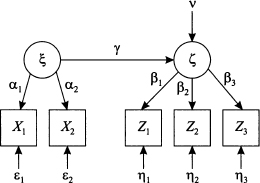
The assumption that these variables are somehow related makes sense, but unfortunately they are not directly observable; they are latent variables. Nevertheless, imagine that we wish to build a model expressing the dependence between latent variables. For instance, we may consider the structural equation

where ζ and ζ are latent variables, v is an error term, and γ is an unknown parameter. If we want to estimate the parameter, we need to relate the latent variables to observable variables, which play the role of measurements. Imagine that the latent variable ζ can be related to observable variables X1 and X2 by the following measurement model:

where α1 and α2 are unknown parameters, and 1 and 2 are errors. This is an interdependence model, quite similar to factor analysis. By the same token, the measurement model for ζ can be something like

The overall model can be depicted as in Fig. 15.4. We stress again that a structural model with latent variables includes both dependence and interdependence components. Methods have been proposed to estimate the unknown parameters, combining ideas from regression and factor analysis.
Fig. 15.4 Schematic illustration of a structural model with latent variables.
15.2.8 Multidimensional scaling
Multidimensional scaling is a family of procedures that aim at producing a low-dimensional representation of object similarity/dissimilarity. Consider n brands and a similarity matrix, whose entry dij measures the distance between brands i and j, as perceived by consumers. This matrix is a direct input of multidimensional scaling, whereas other methods aim at computing distances. Then, we want to find a representation of brands as points on a plane, in such a way that the geometric (Euclidean) distance δij between points is approximately proportional to the perceived distance between brands:

for some irrelevant constant α. The idea is illustrated in Fig. 15.5. In a marketing context, for instance, multidimensional scaling can help researchers to understand how consumers perceive brands and how product features relate to each other. We observe that multidimensional scaling procedures accomplish a form of dimensionality reduction, are exploratory in nature, and can be classified as interdependence methods.
Fig. 15.5 Schematic illustration of multidimensional scaling.

Table 15.2 Correspondence analysis works on a two-way contingency table.
15.2.9 Correspondence analysis
Correspondence analysis is a graphical technique for representing the information included in a two-way contingency table containing frequency counts. For example, Table 15.2 lists the number of times an attribute (crispy, sugar-free, good with coffee, etc.) is used by consumers to describe a snack (cookies, candies, muffins, etc.).5 The method deals with two categorical or discrete quantitative variables and aims at visualizing how row and column profiles relate to each other, by developing indexes that are used as coordinates for depicting row and column categories on a plane. Again, this can be used for assessing product positioning, among other things. Correspondence analysis is another exploratory- interdependence method, which can be considered as a factorial decomposition of a contingency table.
This cursory and superficial overview should illustrate well the richness of multivariate analysis and its potential for applications. We should also mention that:
- The boundaries between multivariate analysis tools are not quite sharp, as some methods can be considered as specific cases of other methods.
- Methods can be combined in practice. For instance, in order to ease the task of a cluster analysis algorithm, we may first reduce problem dimensionality by principal component analysis.
15.3 MATRIX ALGEBRA AND MULTIVARIATE ANALYSIS
The methods that we describe in the next two chapters rely heavily on matrices and linear algebra, which we have covered in Chapter 3. In this section we discuss a few more concepts that are useful in multivariate analysis. Unfortunately, when moving to multivariate statistics, we run out of notation. As usual, capital letters will refer to random quantities, with boldface reserved for random vectors such as X and Z; elements of these vectors will be denoted by Xi and Zi, and scalar random variables will be denoted by Y as usual. Lowercase letters, such as x and x, refer to numbers or specific realizations of random quantities X and x, respectively. We will also use matrices such as Σ, S, and A; usually, there is no ambiguity between matrices and random vectors. However, we also need to represent the whole set of observations in matrix form. Observation k is a vector X(k) p, with elements Xj(k), j = 1, …, p, corresponding to single variables or dimensions. Observations are typically collected into matrices, where columns correspond to single variables and rows to their joint realizations (observations). The whole dataset will be denoted by χ, to avoid confusion with vector X. The element [χ]kj in row k and column j of the data matrix is the element j of observation k, i.e., Xj(k):
For instance, by using the data matrix χ, we may express the column vector of sample means in the compact form

Here, 1n n is a column vector with n elements set to 1, not to be confused with the identity matrix In n,n. A useful matrix is
Example 15.3 (The centering matrix) When we premultiply a vector X n, consisting of univariate observations X1, …, Xn, by the matrix
we are subtracting the sample mean  from all elements of X:
Not surprisingly, the matrix Hn is called centering matrix and may be used with a data matrix χ in order to obtain the matrix of centered data

To understand how this last formula works, you should think of the data matrix as a bundle of column vectors, each one corresponding to a single variable.
15.3.1 Covariance matrices
Given a random vector X p with expected value μ, the covariance matrix can be expressed as
Note that inside the expectation we are multiplying a column vector p x 1 and a row vector 1 x p, which does result in a square matrix p x p. It may also be worth noting that there is a slight inconsistency of notation, since we denote variance in the scalar case by σ2, but we do not use Σ2 here, as this would be somewhat confusing. The element in row i and column j of matrix Σ, [Σ]ij, is the covariance σij between Xi and Xj. Consistently, we should regard the variance of Xi as Cov(Xi, Xi) = σii. We may also express the covariance matrix as
This is just a vector generalization of Eq. (8.5). If we consider a linear combination Z of variables X, i.e.,

then the variance of Z is
(15.2) 
where Σ is the covariance matrix of X. By a similar token, let us consider a linear transformation from random vector X to random vector Z, represented by the matrix A, i.e.

It turns out6 that the covariance matrix of Z is

By recalling that a linear combination of jointly normal variables is normal, the following theorem can be immediately understood.
THEOREM 15.1 Let X be a vector of n jointly normal variables with expected value μ and covariance matrix Σ. Given a matrix A m,n, the transformed vector AX, taking values in m, has a jointly normal distribution with expected value Aμ and covariance matrix AΣAT.
The above properties refer to covariance matrices, i.e., to probabilistic concepts. The same results carry over to the sample covariance matrix, which we denote by S. Again, there is a bit of notational inconsistency with respect to sample variance S2 in the scalar case, but we will think of sample variance in terms of sample covariance, Sj2 = Sjj, and adopt this notation, which is consistent with the use of Σ for a covariance matrix. The sample covariance matrix may be expressed in terms of random observation vectors X(k):
The expression in Eq. (15.4) is a multivariable generalization of the familiar way of rewriting sample variance; see Eq. (9.7). It is also fairly easy to show that we may write the sample covariance matrix in a very compact form using the data matrix χ. The sum in Eq. (15.4) can be expressed as χTχ, and by rewriting the vector of sample means as in Eq. (15.1) we obtain
From a computational point of view, Eq. (15.5) may not be quite convenient; however, these ways of rewriting the sample covariance matrix may come in handy when proving theorems and analyzing data manipulations. If the data are already centered, then expressing the sample covariance matrix is immediate:
We should also note the following properties, that generalize what we are familiar with in the scalar case:
(15.6) 

where b is an arbitrary vector of real numbers.
If we need the sample correlation matrix R, consisting of sample correlation coefficients Rij between Xi and Xj, we may introduce the diagonal matrix of sample standard deviations
and then let

15.3.2 Measuring distance and the Mahalanobis transformation
In Section 3.3.1 we defined the concept of vector norm, which can be used to measure the distance between points in p. We might also define the distance between observed vectors in the same way, but in statistics we typically want to account for the covariance structure as well. As an introduction, consider the distance between the realization of a random variable X and its expected value μ, or between two realizations X1 and X2. Does a distance measure based on a plain difference, such as |X - μ| or |X1 - X2|, make sense? Such a measure is highly debatable, from a statistical perspective, as it disregards dispersion altogether. A suitable measure should be expressed in terms of number of standard deviations, which leads to the standardized distances
Alternatively, we may consider the squared distances

To generalize the idea to the distance between observation vectors X(1) and X(2), we may rely on the covariance matrix and define the squared distance

where Σ-1 is the inverse of the covariance matrix. More often than not, we do not know the underlying covariance matrix, and we have to replace it with the sample covariance matrix S. We may also express the distance with respect to the expected value in the same way:

The last expression should be familiar, since it is related to the argument of the exponential function that defines the joint PDF of a multivariate normal distribution.7 We also recall that the level curves of this PDF are ellipses, whose shape depends on the correlation between variables. This is very helpful in understanding the rationale behind the definition of the distances described above, which are known as Mahalanobis distances. Consider the two points A and B in Fig. 15.6. The figure is best interpreted in terms of a bivariate normal distribution with expected value μ; the ellipse is a level curve of its PDF. Geometrically, if we consider standard Euclidean distance, the points A and B do not have the same distance from μ. However, if we account for covariance by Mahalanobis distance, we see that the two points have the same distance from μ. Strictly speaking, we cannot compare the probabilities of outcomes A and B, as they are both zero; nevertheless, the two points are on the same “isodensity” curve and are, in a loose sense, equally likely.
Fig. 15.6 Illustration of Mahalanobis distance.

Mahalanobis distance can also be interpreted as a Euclidean distance modified by a suitably chosen weight matrix, which changes the relative importance of dimensions. Measuring distances is essential in clustering algorithms, as we will see in Section 17.4.1. Finally, Mahalanobis distance may also be interpreted in terms of a transformation, called Mahalanobis transformation. Consider the square root of the covariance matrix, i.e., a symmetric matrix Σ1/2 such that

and the transformation
where X is a random variable with expected value μ and covariance matrix Σ. Clearly, this transformation is just an extension of familiar standardization of a scalar random variable. The distance between X and μ can be expressed in terms of standardized variables as follows:
Now, using Eqs. (15.3) and (15.7), we find that the covariance matrix of the standardized variables is
Thus, we see that Mahalanobis transformation yields a set of uncorrelated and standardized variables.
For further reading
- The theory behind multivariate analysis may be rather challenging, but a readable treatment can be found in Refs. [1] and [5].
- See Chapter 1 of Ref. [6] for a discussion of dependence vs. interdependence techniques, as well as the different types of scale.
- One of the most fertile application domains of multivariate methods is marketing; see Ref. [4] for an illustration of this kind of applications.
- A very nice compromise between the need of explaining the theory behind the methods, which is the only way of truly understanding their pitfalls, and the urge of presenting concrete and real-life applications has been struck in the book by Lattin et al. [3].
- The link between matrix algebra and multivariate statistics is well documented in the treatise by Harville [2].
REFERENCES
1. W. Härdle and L. Simar, Applied Multivariate Statistical Analysis, 2nd ed., Springer, Berlin, 2007.
2. D.H. Harville, Matrix Algebra from a Statistician’s Perspective, Springer, New York, 1997.
3. J.M. Lattin, J.D. Carroll, and P.E. Green, Analyzing Multivariate Data, Brooks/Cole, Belmont, CA, 2003.
4. J.H. Myers and G.M. Mullet, Managerial Applications of Multivariate Analysis in Marketing, South-Western, Cincinnati, OH, 2003.
5. A.C. Rencher, Methods of Multivariate Analysis, 2nd ed., Wiley, New York, 2002.
6. S. Sharma, Applied Multivariate Techniques, Wiley, Hoboken, NJ, 1996.
1 See Section 4.4.1.
2 This is likely to stem from our struggle with many suitcases that do not like the idea of fitting the trunk of our cheap car.
3 The case was an investigation of city logistics in Turin and Piedmont Region, carried out by a colleague of mine. And if you think that a more thorough interview technique would solve the issue, try stopping a voluminous truck driver, at 8 a.m., in the middle of a congested road, for a long and amicable conversation. Needless to say, “voluminous” refers to the driver.
4 See Section 4.1.1.
5 For a complete example, see p. 311 of the book by Myers and Mullen [4].
6 See Chapter 3 of the textbook by Rencher [5] for a detailed treatment.
7 See Section 8.4.