CHAPTER 4

Tracking the Pathways to Success

IF A GAMBLER of Cardano’s day had understood Cardano’s mathematical work on chance, he could have made a tidy profit betting against less sophisticated players. Today, with what he had to offer, Cardano could have achieved both fame and fortune writing books like The Idiot’s Guide to Casting Dice with Suckers. But in his own time, Cardano’s work made no big splash, and his Book on Games of Chance remained unpublished until long after his death. Why did Cardano’s work have so little impact? As we’ve said, one hindrance to those who preceded him was the lack of a good system of algebraic notation. That system in Cardano’s day was improving but was still in its infancy. Another roadblock, however, had yet to be removed: Cardano worked at a time when mystical incantation was more valued than mathematical calculation. If people did not look for the order in nature and did not develop numerical descriptions of events, then a theory of the effect of randomness on those events was bound to go unappreciated. As it turned out, had Cardano lived just a few decades later, both his work and its reception might have been far different, for the decades after his death saw the unfolding of historic changes in European thought and belief, a transformation that has traditionally been dubbed the scientific revolution.

The scientific revolution was a revolt against a way of thinking that was prevalent as Europe emerged from the Middle Ages, an era in which people’s beliefs about the way the world worked were not scrutinized in any systematic manner. Merchants in one town stole the clothes off a hanged man because they believed it would help their sales of beer. Parishioners in another believed illness could be cured by chanting sacrilegious prayers as they marched naked around their church altar.¹ One trader even believed that relieving himself in the “wrong” toilet would bring bad fortune. Actually he was a bond trader who confessed his secret to a CNN reporter in 2003.² Yes, some people still adhere to superstitions today, but at least today, for those who are interested, we have the intellectual tools to prove or disprove the efficacy of such actions. But if Cardano’s contemporaries, say, won at dice, rather than analyzing their experience mathematically, they would say a prayer of thanks or refuse to wash their lucky socks. Cardano himself believed that streaks of losses occur because “fortune is averse” and that one way to improve your results is to give the dice a good hard throw. If a lucky 7 is all in the wrist, why stoop to mathematics?

The moment that is often considered the turning point for the scientific revolution came in 1583, just seven years after Cardano’s death. That is when a young student at the University of Pisa sat in a cathedral and, according to legend, rather than listening to the services, stared at something he found far more intriguing: the swinging of a large hanging lamp. Using his pulse as a timer, Galileo Galilei noticed that the lamp seemed to take the same amount of time to swing through a wide arc as it did to swing through a narrow one. That observation suggested to him a law: the time required by a pendulum to perform a swing is independent of the amplitude of the swing. Galileo’s was a precise and practical observation, and although simple, it signified a new approach to the description of physical phenomena: the idea that science must focus on experience and experimentation—how nature operates—rather than on what intuition dictates or our minds find appealing. And most of all, it must be done with mathematics.

Galileo employed his scientific skills to write a short piece on gambling, “Thoughts about Dice Games.” The work was produced at the behest of his patron, the grand duke of Tuscany. The problem that bothered the grand duke was this: when you throw three dice, why does the number 10 appear more frequently than the number 9? The excess of 10s is only about 8 percent, and neither 10 nor 9 comes up very often, so the fact that the grand duke played enough to notice the small difference means he probably needed a good twelve-step program more than he needed Galileo. For whatever reason, Galileo was not keen to work on the problem and grumbled about it. But like any consultant who wants to stay employed, he kept his grumbling low-key and did his job.

If you throw a single die, the chances of any number in particular coming up are 1 in 6. But if you throw two dice, the chances of different totals are no longer equal. For example, there is a 1 in 36 chance of the dice totaling 2 but twice that chance of their totaling 3. The reason is that a total of 2 can be obtained in only 1 way, by tossing two 1s, but a total of 3 can be obtained in 2 ways, by tossing a 1 and then a 2 or a 2 and then a 1. That brings us to the next big step in understanding random processes, which is the subject of this chapter: the development of systematic methods for analyzing the number of ways in which events can happen.

         

THE KEY TO UNDERSTANDING the grand duke’s confusion is to approach the problem as if you were a Talmudic scholar: rather than attempting to explain why 10 comes up more frequently than 9, we ask, why shouldn’t 10 come up more frequently than 9? It turns out there is a tempting reason to believe that the dice should sum to 10 and 9 with equal frequency: both 10 and 9 can be constructed in 6 ways from the throw of three dice. For 9 we can write those ways as (621), (531), (522), (441), (432), and (333). For 10 they are (631), (622), (541), (532), (442), and (433). According to Cardano’s law of the sample space, the probability of obtaining a favorable outcome is equal to the proportion of outcomes that are favorable. A sum of 9 and 10 can be constructed in the same number of ways. So why is one more probable than the other?

The reason is that, as I’ve said, the law of the sample space in its original form applies only to outcomes that are equally probable, and the combinations listed above are not. For instance, the outcome (631)—that is, throwing a 6, a 3, and a 1—is 6 times more likely than the outcome (333) because although there is only 1 way you can throw three 3s, there are 6 ways you can throw a 6, a 3, and a 1: you can throw a 6 first, then a 3, and then a 1, or you can throw a 1 first, then a 3, then a 6, and so on. Let’s represent an outcome in which we are keeping track of the order of throws by a triplet of numbers separated by commas. Then the short way of saying what we just said is that the outcome (631) consists of the possibilities (1,3,6), (1,6,3), (3,1,6), (3,6,1), (6,1,3), and (6,3,1), whereas the outcome (333) consists only of (3,3,3). Once we’ve made this decomposition, we can see that the outcomes are equally probable and we can apply the law. Since there are 27 ways of rolling a 10 with three dice but only 25 ways to get a total of 9, Galileo concluded that with three dice, rolling a 10 was 27/25, or about 1.08, times more likely.

In solving the problem, Galileo implicitly employed our next important principle: The chances of an event depend on the number of ways in which it can occur. That is not a surprising statement. The surprise is just how large that effect is—and how difficult it can be to calculate. For example, suppose you give a 10-question true-or-false quiz to your class of 25 sixth-graders. Let’s do an accounting of the results a particular student might achieve: she could answer all questions correctly; she could miss 1 question—that can happen in 10 ways because there are 10 questions she could miss; she could miss a pair of questions—that can happen in 45 ways because there are 45 distinct pairs of questions; and so on. As a result, on average in a collection of students who are randomly guessing, for every student scoring 100 percent, you’ll find about 10 scoring 90 percent and 45 scoring 80 percent. The chances of getting a grade near 50 percent are of course higher still, but in a class of 25 the probability that at least one student will get a B (80 percent) or better if all the students are guessing is about 75 percent. So if you are a veteran teacher, it is likely that among all the students over the years who have shown up unprepared and more or less guessed at your quizzes, some were rewarded with an A or a B.

A few years ago Canadian lottery officials learned the importance of careful counting the hard way when they decided to give back some unclaimed prize money that had accumulated.³ They purchased 500 automobiles as bonus prizes and programmed a computer to determine the winners by randomly selecting 500 numbers from their list of 2.4 million subscriber numbers. The officials published the unsorted list of 500 winning numbers, promising an automobile for each number listed. To their embarrassment, one individual claimed (rightly) that he had won two cars. The officials were flabbergasted—with over 2 million numbers to choose from, how could the computer have randomly chosen the same number twice? Was there a fault in their program?

The counting problem the lottery officials ran into is equivalent to a problem called the birthday problem: how many people must a group contain in order for there to be a better than even chance that two members of the group will share the same birthday (assuming all birth dates are equally probable)? Most people think the answer is half the number of days in a year, or about 183. But that is the correct answer to a different question: how many people do you need to have at a party for there to be a better than even chance that one of them will share your birthday? If there is no restriction on which two people will share a birthday, the fact that there are many possible pairs of individuals who might have shared birthdays changes the answer drastically. In fact, the answer is astonishingly low: just 23. When pulling from a pool of 2.4 million, as in the case of the Canadian lottery, it takes many more than 500 numbers to have an even chance of a repeat. But still that possibility should not have been ignored. The chances of a match come out, in fact, to about 5 percent. Not huge, but it could have been accounted for by having the computer cross each number off the list as it was chosen. For the record, the Canadian lottery requested the lucky fellow to forgo the second car, but he refused.

Another lottery mystery that raised many eyebrows occurred in Germany on June 21, 1995.⁴ The freak event happened in a lottery called Lotto 6/49, which means that the winning six numbers are drawn from the numbers 1 to 49. On the day in question the winning numbers were 15-25-27-30-42-48. The very same sequence had been drawn previously, on December 20, 1986. It was the first time in 3,016 drawings that a winning sequence had been repeated. What were the chances of that? Not as bad as you’d think. When you do the math, the chance of a repeat at some point over the years comes out to around 28 percent.

Since in a random process the number of ways in which an outcome can occur is a key to determining how probable it is, the key question is, how do you calculate the number of ways in which something can occur? Galileo seems to have missed the significance of that question. He did not carry his work on randomness beyond that problem of dice and said in the first paragraph of his work that he was writing about dice only because he had been “ordered” to do so.⁵ In 1633, as his reward for promoting a new approach to science, Galileo was condemned by the Inquisition. But science and theology had parted ways for good; scientists now analyzing how? were unburdened by the theologians’ issue of why? Soon a scholar from a new generation, schooled since his youth on Galileo’s philosophy of science, would take the analysis of contingency counting to new heights, reaching a level of understanding without which most of today’s science could not be conducted.

         

WITH THE BLOSSOMING of the scientific revolution the frontiers of randomness moved from Italy to France, where a new breed of scientist, rebelling against Aristotle and following Galileo, developed it further and deeper than had either Cardano or Galileo. This time the importance of the new work would be recognized, and it would make waves all over Europe. Though the new ideas would again be developed in the context of gambling, the first of this new breed was more a mathematician turned gambler than, like Cardano, a gambler turned mathematician. His name was Blaise Pascal.

Pascal was born in June 1623 in Clermont-Ferrand, a little more than 250 miles south of Paris. Realizing his son’s brilliance, and having moved to Paris, Blaise’s father introduced him at age thirteen to a newly founded discussion group there that insiders called the Académie Mersenne after the black-robed friar who had founded it. Mersenne’s society included the famed philosopher-mathematician René Descartes and the amateur mathematics genius Pierre de Fermat. The strange mix of brilliant thinkers and large egos, with Mersenne present to stir the pot, must have had a great influence on the teenage Blaise, who developed personal ties to both Fermat and Descartes and picked up a deep grounding in the new scientific method. “Let all the disciples of Aristotle…,” he would write, “recognize that experiment is the true master who must be followed in Physics.”⁶

But how did a bookish and stodgy fellow of pious beliefs become involved with issues of the urban gambling scene? On and off Pascal experienced stomach pains, had difficulty swallowing and keeping food down, and suffered from debilitating weakness, severe headaches, bouts of sweating, and partial paralysis of the legs. He stoically followed the advice of his physicians, which involved bleedings, purgings, and the consumption of asses’ milk and other “disgusting” potions that he could barely keep from vomiting—a “veritable torture,” according to his sister Gilberte.⁷ Pascal had by then left Paris, but in the summer of 1647, aged twenty-four and growing desperate, he moved back with his sister Jacqueline in search of better medical care. There his new bevy of doctors offered the state-of-the-art advice that Pascal “ought to give up all continued mental labor, and should seek as much as possible all opportunities to divert himself.”⁸ And so Pascal taught himself to kick back and relax and began to spend time in the company of other young men of leisure. Then, in 1651, Blaise’s father died, and suddenly Pascal was a twenty-something with an inheritance. He put the cash to good use, at least in the sense of his doctors’ orders. Biographers call the years from 1651 to 1654 Pascal’s “worldly period.” His sister Gilberte called it “the time of his life that was worst employed.”⁹ Though he put some effort into self-promotion, his scientific research went almost nowhere, but for the record, his health was the best it had ever been.

Often in history the study of the random has been aided by an event that was itself random. Pascal’s work represents such an occasion, for it was his abandonment of study that led him to the study of chance. It all began when one of his partying pals introduced him to a forty-five-year-old snob named Antoine Gombaud. Gombaud, a nobleman whose title was chevalier de Méré, regarded himself as a master of flirtation, and judging by his catalog of romantic entanglements, he was. But de Méré was also an expert gambler who liked the stakes high and won often enough that some suspected him of cheating. And when he stumbled on a little gambling quandary, he turned to Pascal for help. With that, de Méré initiated an investigation that would bring to an end Pascal’s scientific dry spell, cement de Méré’s own place in the history of ideas, and solve the problem left open by Galileo’s work on the grand duke’s dice-tossing question.

The year was 1654. The question de Méré brought to Pascal was called the problem of points: Suppose you and another player are playing a game in which you both have equal chances and the first player to earn a certain number of points wins. The game is interrupted with one player in the lead. What is the fairest way to divide the pot? The solution, de Méré noted, should reflect each player’s chance of victory given the score that prevails when the game is interrupted. But how do you calculate that?

Pascal realized that whatever the answer, the methods needed to calculate it were yet unknown, and those methods, whatever they were, could have important implications in any type of competitive situation. And yet, as often happens in theoretical research, Pascal found himself unsure of, and even confused about, his plan of attack. He decided he needed a collaborator, or at least another mathematician with whom he could discuss his ideas. Marin Mersenne, the great communicator, had died a few years earlier, but Pascal was still wired into the Académie Mersenne network. And so in 1654 began one of the great correspondences in the history of mathematics, between Pascal and Pierre de Fermat.

In 1654, Fermat held a high position in the Tournelle, or criminal court, in Toulouse. When the court was in session, a finely robed Fermat might be found condemning errant functionaries to be burned at the stake. But when the court was not in session, he would turn his analytic skills to the gentler pursuit of mathematics. He may have been an amateur, but Pierre de Fermat is usually considered the greatest amateur mathematician of all times.

Fermat had not gained his high position through any particular ambition or accomplishment. He achieved it the old-fashioned way, by moving up steadily as his superiors dropped dead of the plague. In fact, when Pascal’s letter arrived, Fermat himself was recovering from a bout of the disease. He had even been reported dead, by his friend Bernard Medon. When Fermat didn’t die, an embarrassed but presumably happy Medon retracted his announcement, but there is no doubt that Fermat had been on the brink. As it turned out, though twenty-two years Pascal’s senior, Fermat would outlive his newfound correspondent by several years.

As we’ll see, the problem of points comes up in any area of life in which two entities compete. In their letters, Pascal and Fermat each developed his own approach and solved several versions of the problem. But it was Pascal’s method that proved simpler—even beautiful—and yet is general enough to be applied to many problems we encounter in our everyday experience. Because the problem of points first arose in a betting situation, I’ll illustrate the problem with an example from the world of sports. In 1996 the Atlanta Braves beat the New York Yankees in the first 2 games of the baseball World Series, in which the first team to win 4 games is crowned champion. The fact that the Braves won the first 2 games didn’t necessarily mean they were the superior team. Still, it could be taken as a sign that they were indeed better. Nevertheless, for our current purposes we will stick to the assumption that either team was equally likely to win each game and that the first 2 games just happened to go to the Braves.

Given that assumption, what would have been fair odds for a bet on the Yankees—that is, what was the chance of a Yankee comeback? To calculate it, we count all the ways in which the Yankees could have won and compare that to the number of ways in which they could have lost. Two games of the series had been played, so there were 5 possible games yet to play. And since each of those games had 2 possible outcomes—a Yankee win (Y) or a Braves win (B)—there were 2⁵, or 32, possible outcomes. For instance, the Yankees could have won 3, then lost 2: YYYBB; or they could have alternated victories: YBYBY. (In the latter case, since the Braves would have won 4 games with the 6th game, the last game would never have been played, but we’ll get to that in a minute.) The probability that the Yankees would come back to win the series was equal to the number of sequences in which they would win at least 4 games divided by the total number of sequences, 32; the chance that the Braves would win was equal to the number of sequences in which they would win at least 2 more games also divided by 32.

This calculation may seem odd, because as I mentioned, it includes scenarios (such as YBYBY) in which the teams keep playing even after the Braves have won the required 4 games. The teams would certainly not play a 7th game once the Braves had won 4. But mathematics is independent of human whim, and whether or not the players play the games does not affect the fact that such sequences exist. For example, suppose you’re playing a coin-toss game in which you win if at any time heads come up. There are 2², or 4, possible two-toss sequences: HT, HH, TH, and TT. In the first two of these, you would not bother tossing the coin again because you would already have won. Still, your chances of winning are 3 in 4 because 3 of the 4 complete sequences include an H.

So in order to calculate the Yankees’ and the Braves’ chances of victory, we simply make an accounting of the possible 5-game sequences for the remainder of the series. First, the Yankees would have been victorious if they had won 4 of the 5 possible remaining games. That could have happened in 1 of 5 ways: BYYYY, YBYYY, YYBYY, YYYBY, or YYYYB. Alternatively, the Yankees would have triumphed if they had won all 5 of the remaining games, which could have happened in only 1 way: YYYYY. Now for the Braves: they would have become champions if the Yankees had won only 3 games, which could have happened in 10 ways (BBYYY, BYBYY, and so on), or if the Yankees had won only 2 games (which again could have happened in 10 ways), or if the Yankees had won only 1 game (which could have happened in 5 ways), or if they had won none (which could have happened in only 1 way). Adding these possible outcomes together, we find that the chance of a Yankees victory was 6 in 32, or about 19 percent, versus 26 in 32, or about 81 percent for the Braves. According to Pascal and Fermat, if the series had abruptly been terminated, that’s how they should have split the bonus pot, and those are the odds that should have been set if a bet was to be made after the first 2 games. For the record, the Yankees did come back to win the next 4 games, and they were crowned champion.

The same reasoning could also be applied to the start of the series—that is, before any game has been played. If the two teams have equal chances of winning each game, you will find, of course, that they have an equal chance of winning the series. But similar reasoning works if they don’t have an equal chance, except that the simple accounting I just employed would have to be altered slightly: each outcome would have to be weighted by a factor describing its relative probability. If you do that and analyze the situation at the start of the series, you will discover that in a 7-game series there is a sizable chance that the inferior team will be crowned champion. For instance, if one team is good enough to warrant beating another in 55 percent of its games, the weaker team will nevertheless win a 7-game series about 4 times out of 10. And if the superior team could be expected to beat its opponent, on average, 2 out of each 3 times they meet, the inferior team will still win a 7-game series about once every 5 matchups. There is really no way for sports leagues to change this. In the lopsided ²/₃-probability case, for example, you’d have to play a series consisting of at minimum the best of 23 games to determine the winner with what is called statistical significance, meaning the weaker team would be crowned champion 5 percent or less of the time (see chapter 5). And in the case of one team’s having only a 55–45 edge, the shortest statistically significant “world series” would be the best of 269 games, a tedious endeavor indeed! So sports playoff series can be fun and exciting, but being crowned “world champion” is not a very reliable indication that a team is actually the best one.

As I said, the same reasoning applies to more than games, gambling, and sports. For example, it shows that if two companies compete head-to-head or two employees within a company compete, though there may be a winner and a loser each quarter or each year, to get a reliable answer regarding which company or which employee is superior by simply tallying who beats whom, you’d have to make the comparison over decades or centuries. If, for instance, employee A is truly superior and would in the long run win a performance comparison with employee B on 60 out of 100 occasions, in a simple best-of-5 series of comparisons the weaker employee will still win almost one-third of the time. It is dangerous to judge ability by short-term results.

The counting in all these problems has been simple enough to carry out without much effort. But when the numbers are higher, the counting becomes difficult. Consider, for example, this problem: You are arranging a wedding reception for 100 guests, and each table seats 10. You can’t sit your cousin Rod with your friend Amy because eight years ago they had an affair and she dumped him. On the other hand, both Amy and Leticia want to sit next to your buff cousin Bobby, and your aunt Ruth had better be at a table out of earshot or the dueling flirtations will be gossip fodder for holiday dinners for the next five years. You carefully consider the possibilities. Take just the first table. How many ways are there to choose 10 people from a group of 100? That’s the same question as, in how many ways can you apportion 10 investments among 100 mutual funds or 10 germanium atoms among 100 locations in a silicon crystal? It’s the type of problem that comes up repeatedly in the theory of randomness, and not only in the problem of points. But with larger numbers it is tedious or impossible to count the possibilities by listing them explicitly. That was Pascal’s real accomplishment: a generally applicable and systematic approach to counting that allows you to calculate the answer from a formula or read it off a chart. It is based on a curious arrangement of numbers in the shape of a triangle.

         

THE COMPUTATIONAL METHOD at the heart of Pascal’s work was actually discovered by a Chinese mathematician named Jia Xian around 1050, published by another Chinese mathematician, Zhu Shijie, in 1303, discussed in a work by Cardano in 1570, and plugged into the greater whole of probability theory by Pascal, who ended up getting most of the credit.¹⁰ But the prior work didn’t bother Pascal. “Let no one say I have said nothing new,” Pascal argued in his autobiography. “The arrangement of the subject is new. When we play tennis, we both play with the same ball, but one of us places it better.”¹¹ The graphic invention employed by Pascal, given below, is thus called Pascal’s triangle. In the figure, I have truncated Pascal’s triangle at the tenth row, but it can be continued downward indefinitely. In fact, it is easy to continue the triangle, for with the exception of the 1 at the apex, each number is the sum of the number in the line above it to the left and the number in the line above it to the right (add a 0 if there is no number in the line above it to the left or to the right).

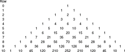
Pascal’s triangle

Pascal’s triangle is useful any time you need to know the number of ways in which you can choose some number of objects from a collection that has an equal or greater number. Here is how it works in the case of the wedding guests: To find the number of distinct seatings of 10 you can form from a group of 100 guests, you would start by looking down the numbers to the left of the triangle until you found the row labeled 100. The triangle I supplied does not go down that far, but for now let’s pretend it does. The first number in row 100 tells you the number of ways you can choose 0 guests from a group of 100. There is just 1 way, of course: you simply don’t choose anyone. That is true no matter how many total guests you are choosing from, which is why the first number in every row is a 1. The second number in row 100 tells you the number of ways you can choose 1 guest from the group of 100. There are 100 ways to do that: you can choose just guest number 1, or just guest number 2, and so on. That reasoning applies to every row, and so the second number in each row is simply the number of that row. The third number in each row represents the number of distinct groups of 2 you can form, and so on. The number we seek—the number of distinct arrangements of 10 you can form—is therefore the eleventh number in the row. Even if I had extended the triangle to include 100 rows, that number would be far too large to put on the page. In fact, when some wedding guest inevitably complains about the seating arrangements, you might point out how long it would have taken you to consider every possibility: assuming you spent one second considering each one, it would come to roughly 10,000 billion years. The unhappy guest will assume, of course, that you are being histrionic.

In order for us to use Pascal’s triangle, let’s say for now that your guest list consists of just 10 guests. Then the relevant row is the one at the bottom of the triangle I provided, labeled 10. The numbers in that row represent the number of distinct tables of 0, 1, 2, and so on, that can be formed from a collection of 10 people. You may recognize these numbers from the sixth-grade quiz example—the number of ways in which a student can get a given number of problems wrong on a 10-question true-or-false test is the same as the number of ways in which you can choose guests from a group of 10. That is one of the reasons for the power of Pascal’s triangle: the same mathematics can be applied to many different situations. For the Yankees-Braves World Series example, in which we tediously counted all the possibilities for the remaining 5 games, we can now read the number of ways in which the Yankees can win 0, 1, 2, 3, 4, or 5 games directly from row 5 of the triangle:

         

1                   5                   10                   10                   5                   1

         

We can see at a glance that the Yankees’ chance of winning 2 games (10 ways) was twice as high as their chance of winning 1 game (5 ways).

Once you learn the method, applications of Pascal’s triangle crop up everywhere. A friend of mine once worked for a start-up computer-games company. She would often relate how, although the marketing director conceded that small focus groups were suited for “qualitative conclusions only,” she nevertheless sometimes reported an “overwhelming” 4-to-2 or 5-to-1 agreement among the members of the group as if it were meaningful. But suppose you hold a focus group in which 6 people will examine and comment on a new product you are developing. Suppose that in actuality the product appeals to half the population. How accurately will this preference be reflected in your focus group? Now the relevant line of the triangle is the one labeled 6, representing the number of possible subgroups of 0, 1, 2, 3, 4, 5, or 6 whose members might like (or dislike) your product:

         

1                   6                   15                   20                   15                   6                   1

         

From these numbers we see that there are 20 ways in which the group members could split 50/50, accurately reflecting the views of the populace at large. But there are also 1 + 6 + 15 + 15 + 6 + 1 = 44 ways in which you might find an unrepresentative consensus, either for or against. So if you are not careful, the chances of being misled are 44 out of 64, or about two-thirds. This example does not prove that if agreement is achieved, it is random. But neither should you assume that it is significant.

Pascal and Fermat’s analysis proved to be a big first step in a coherent mathematical theory of randomness. The final letter of their famous exchange is dated October 27, 1654. A few weeks later Pascal sat in a trance for two hours. Some call that trance a mystical experience. Others lament that he had finally blasted off from planet Sanity. However you describe it, Pascal emerged from the event a transformed man. It was a transformation that would lead him to make one more fundamental contribution to the concept of randomness.

         

IN 1662, a few days after Pascal died, a servant noticed a curious bulge in one of Pascal’s jackets. The servant pulled open the lining to find hidden within it folded sheets of parchment and paper. Pascal had apparently carried them with him every day for the last eight years of his life. Scribbled on the sheets, in his handwriting, was a series of isolated words and phrases dated November 23, 1654. The writings were an emotional account of the trance, in which he described how God had come to him and in the space of two hours delivered him from his corrupt ways.

Following that revelation, Pascal had dropped most of his friends, calling them “horrible attachments.”¹² He sold his carriage, his horses, his furniture, his library—everything except his Bible. He gave his money to the poor, leaving himself with so little that he often had to beg or borrow to obtain food. He wore an iron belt with points on the inside so that he was in constant discomfort and pushed the belt’s spikes into his flesh whenever he found himself in danger of feeling happy. He denounced his studies of mathematics and science. Of his childhood fascination with geometry, he wrote, “I can scarcely remember that there is such a thing as geometry. I recognize geometry to be so useless…it is quite possible I shall never think of it again.”¹³

Yet Pascal remained productive. In the years that followed the trance, he recorded his thoughts about God, religion, and life. Those thoughts were later published in a book titled Pensées, a work that is still in print today. And although Pascal had denounced mathematics, amid his vision of the futility of the worldly life is a mathematical exposition in which he trained his weapon of mathematical probability squarely on a question of theology and created a contribution just as important as his earlier work on the problem of points.

The mathematics in Pensées is contained in two manuscript pages covered on both sides by writing going in every direction and full of erasures and corrections. In those pages, Pascal detailed an analysis of the pros and cons of one’s duty to God as if he were calculating mathematically the wisdom of a wager. His great innovation was his method of balancing those pros and cons, a concept that is today called mathematical expectation.

Pascal’s argument went like this: Suppose you concede that you don’t know whether or not God exists and therefore assign a 50 percent chance to either proposition. How should you weigh these odds when deciding whether to lead a pious life? If you act piously and God exists, Pascal argued, your gain—eternal happiness—is infinite. If, on the other hand, God does not exist, your loss, or negative return, is small—the sacrifices of piety. To weigh these possible gains and losses, Pascal proposed, you multiply the probability of each possible outcome by its payoff and add them all up, forming a kind of average or expected payoff. In other words, the mathematical expectation of your return on piety is one-half infinity (your gain if God exists) minus one-half a small number (your loss if he does not exist). Pascal knew enough about infinity to know that the answer to this calculation is infinite, and thus the expected return on piety is infinitely positive. Every reasonable person, Pascal concluded, should therefore follow the laws of God. Today this argument is known as Pascal’s wager.

Expectation is an important concept not just in gambling but in all decision making. In fact, Pascal’s wager is often considered the founding of the mathematical discipline of game theory, the quantitative study of optimal decision strategies in games. I must admit I find such thinking addictive, and so I sometimes carry it a bit too far. “How much does that parking meter cost?” I ask my son. The sign says 25¢. Yes, but 1 time in every 20 or so visits, I come back late and find a ticket, which runs $40, so the 25¢ cost of the meter is really just a cruel lure, I explain, because my real cost is $2.25. (The extra $2 comes from my 1 in 20 chance of getting a ticket multiplied by its $40 cost.) “How about our driveway,” I ask my other son, “is it a toll road?” Well, we’ve lived at the house about 5 years, or roughly 2,400 times of backing down the driveway, and 3 times I’ve clipped my mirror on the protruding fence post at $400 a shot. You may as well put a toll box out there and toss in 50¢ each time you back up, he tells me. He understands expectation. (He also recommends that I refrain from driving them to school before I’ve had my morning coffee.)

Looking at the world through the lens of mathematical expectation, one often comes upon surprising results. For example, a recent sweepstakes sent through the mail offered a grand prize of $5 million.¹⁴ All you had to do to win was mail in your entry. There was no limit on how many times you could enter, but each entry had to be mailed in separately. The sponsors were apparently expecting about 200 million entries, because the fine print said that the chances of winning were 1 in 200 million. Does it pay to enter this kind of “free sweepstakes offer”? Multiplying the probability of winning times the payoff, we find that each entry was worth ¹/₄₀ of $1, or 2.5¢—far less than the cost of mailing it in. In fact, the big winner in this contest was the post office, which, if the projections were correct, made nearly $80 million in postage revenue on all the submissions.

Here’s another crazy game. Suppose the state of California made its citizens the following offer: Of all those who pay the dollar or two to enter, most will receive nothing, one person will receive a fortune, and one person will be put to death in a violent manner. Would anyone enroll in that game? People do, and with enthusiasm. It is called the state lottery. And although the state does not advertise it in the manner in which I have described it, that is the way it works in practice. For while one lucky person wins the grand prize in each game, many millions of other contestants drive to and from their local ticket vendors to purchase their tickets, and some die in accidents along the way. Applying statistics from the National Highway Traffic Safety Administration and depending on such assumptions as how far each individual drives, how many tickets he or she buys, and how many people are involved in a typical accident, you find that a reasonable estimate of those fatalities is about one death per game.

State governments tend to ignore arguments about the possible bad effects of lotteries. That’s because, for the most part, they know enough about mathematical expectation to arrange that for each ticket purchased, the expected winnings—the total prize money divided by the number of tickets sold—is less than the cost of the ticket. This generally leaves a tidy difference that can be diverted to state coffers. In 1992, however, some investors in Melbourne, Australia, noticed that the Virginia Lottery violated this principle.¹⁵ The lottery involved picking 6 numbers from 1 to 44. Pascal’s triangle, should we find one that goes that far, would show that there are 7,059,052 ways of choosing 6 numbers from a group of 44. The lottery jackpot was $27 million, and with second, third, and fourth prizes included, the pot grew to $27,918,561. The clever investors reasoned, if they bought one ticket with each of the possible 7,059,052 number combinations, the value of those tickets would equal the value of the pot. That made each ticket worth about $27.9 million divided by 7,059,052, or about $3.95. For what price was the state of Virginia, in all its wisdom, selling the tickets? The usual $1.

The Australian investors quickly found 2,500 small investors in Australia, New Zealand, Europe, and the United States willing to put up an average of $3,000 each. If the scheme worked, the yield on that investment would be about $10,800. There were some risks in their plan. For one, since they weren’t the only ones buying tickets, it was possible that another player or even more than one other player would also choose the winning ticket, meaning they would have to split the pot. In the 170 times the lottery had been held, there was no winner 120 times, a single winner only 40 times, and two winners just 10 times. If those frequencies reflected accurately their odds, then the data suggested there was a 120 in 170 chance they would get the pot all to themselves, a 40 in 170 chance they would end up with half the pot, and a 10 in 170 chance they would win just a third of it. Recalculating their expected winnings employing Pascal’s principle of mathematical expectation, they found them to be (120/170 × $27.9 million) + (40/170 × $13.95 million) + (10/170 × $6.975 million) = $23.4 million. That is $3.31 per ticket, a great return on a $1 expenditure even after expenses.

But there was another danger: the logistic nightmare of completing the purchase of all the tickets by the lottery deadline. That could lead to the expenditure of a significant portion of their funds with no significant prize to show for it.

The members of the investment group made careful preparations. They filled out 1.4 million slips by hand, as required by the rules, each slip good for five games. They placed groups of buyers at 125 retail outlets and obtained cooperation from grocery stores, which profited from each ticket they sold. The scheme got going just seventy-two hours before the deadline. Grocery-store employees worked in shifts to sell as many tickets as possible. One store sold 75,000 in the last forty-eight hours. A chain store accepted bank checks for 2.4 million tickets, assigned the work of printing the tickets among its stores, and hired couriers to gather them. Still, in the end, the group ran out of time: they had purchased just 5 million of the 7,059,052 tickets.

Several days passed after the winning ticket was announced, and no one came forward to present it. The consortium had won, but it took its members that long to find the winning ticket. Then, when state lottery officials discovered what the consortium had done, they balked at paying. A month of legal wrangling ensued before the officials concluded they had no valid reason to deny the group. Finally, they paid out the prize.

To the study of randomness, Pascal contributed both his ideas about counting and the concept of mathematical expectation. Who knows what else he might have discovered, despite his renouncing mathematics, if his health had held up. But it did not. In July 1662, Pascal became seriously ill. His physicians prescribed the usual remedies: they bled him and administered violent purges, enemas, and emetics. He improved for a while, and then the illness returned, along with severe headaches, dizziness, and convulsions. Pascal vowed that if he survived, he would devote his life to helping the poor and asked to be moved to a hospital for the incurable, in order that, if he died, he would be in their company. He did die, a few days later, in August 1662. He was thirty-nine. An autopsy found the cause of death to be a brain hemorrhage, but it also revealed lesions in his liver, stomach, and intestines that accounted for the illnesses that had plagued him throughout his life.