CHAPTER 7

Measurement and the Law of Errors

ONE DAY not long ago my son Alexei came home and announced the grade on his most recent English essay. He had received a 93. Under normal circumstances I would have congratulated him on earning an A. And since it was a low A and I know him to be capable of better, I would have added that this grade was evidence that if he put in a little effort, he could score even higher next time. But these were not normal circumstances, and in this case I considered the grade of 93 to be a shocking underestimation of the quality of the essay. At this point you might think that the previous few sentences tell you more about me than about Alexei. If so, you’re right on target. In fact, the above episode is entirely about me, for it was I who wrote Alexei’s essay.

Okay, shame on me. In my defense I should point out that I would normally no sooner write Alexei’s essays than take a foot to the chin for him in his kung fu class. But Alexei had come to me for a critique of his work and as usual presented his request late on the night before the paper was due. I told him I’d get back to him. Proceeding to read it on the computer, I first made a couple of minor changes, nothing worth bothering to note. Then, being a relentless rewriter, I gradually found myself sucked in, rearranging this and rewriting that, and before I finished, not only had he fallen asleep, but I had made the essay my own. The next morning, sheepishly admitting that I had neglected to perform a “save as” on the original, I told him to just go ahead and turn in my version.

He handed me the graded paper with a few words of encouragement. “Not bad,” he told me. “A 93 is really more of an A- than an A, but it was late and I’m sure if you were more awake, you would have done better.” I was not happy. First of all, it is unpleasant when a fifteen-year-old says the very words to you that you have previously said to him, and nevertheless you find his words inane. But beyond that, how could my material—the work of a person whom my mother, at least, thinks of as a professional writer—not make the grade in a high school English class? Apparently I am not alone. Since then I have been told of another writer who had a similar experience, except his daughter received a B. Apparently the writer, with a PhD in English, writes well enough for Rolling Stone, Esquire, and The New York Times but not for English 101. Alexei tried to comfort me with another story: two of his friends, he said, once turned in identical essays. He thought that was stupid and they’d both be suspended, but not only did the overworked teacher not notice, she gave one of the essays a 90 (an A) and the other a 79 (a C). (Sounds odd unless, like me, you’ve had the experience of staying up all night grading a tall stack of papers with Star Trek reruns playing in the background to break the monotony.)

Numbers always seem to carry the weight of authority. The thinking, at least subliminally, goes like this: if a teacher awards grades on a 100-point scale, those tiny distinctions must really mean something. But if ten publishers could deem the manuscript for the first Harry Potter book unworthy of publication, how could poor Mrs. Finnegan (not her real name) distinguish so finely between essays as to award one a 92 and another a 93? If we accept that the quality of an essay is somehow definable, we must still recognize that a grade is not a description of an essay’s degree of quality but rather a measurement of it, and one of the most important ways randomness affects us is through its influence on measurement. In the case of the essay the measurement apparatus was the teacher, and a teacher’s assessment, like any measurement, is susceptible to random variance and error.

Voting is also a kind of measurement. In that case we are measuring not simply how many people support each candidate on election day but how many care enough to take the trouble to vote. There are many sources of random error in this measurement. Some legitimate voters might find that their name is not on the rolls of registered voters. Others mistakenly vote for a candidate other than the one intended. And of course there are errors in counting the votes. Some ballots are improperly accepted or rejected; others are simply lost. In most elections the sum of all these factors doesn’t add up to enough to affect the outcome. But in close elections it can, and then we usually go through one or more recounts, as if our second or third counting of the votes will be less affected by random errors than our first.

In the 2004 governor’s race in the state of Washington, for example, the Democratic candidate was eventually declared the winner although the original tally had the Republican winning by 261 votes out of about 3 million.¹ Since the original vote count was so close, state law required a recount. In that count the Republican won again, but by only 42 votes. It is not known whether anyone thought it was a bad sign that the 219-vote difference between the first and second vote counts was several times larger than the new margin of victory, but the upshot was a third vote count, this one entirely “by hand.” The 42-vote victory amounted to an edge of just 1 vote out of each 70,000 cast, so the hand-counting effort could be compared to asking 42 people to count from 1 to 70,000 and then hoping they averaged less than 1 mistake each. Not surprisingly, the result changed again. This time it favored the Democrat by 10 votes. That number was later changed to 129 when 700 newly discovered “lost votes” were included.

Neither the vote-counting process nor the voting process is perfect. If, for instance, owing to post office mistakes, 1 in 100 prospective voters didn’t get the mailer with the location of the polling place and 1 in 100 of those people did not vote because of it, in the Washington election that would have amounted to 300 voters who would have voted but didn’t because of government error. Elections, like all measurements, are imprecise, and so are the recounts, so when elections come out extremely close, perhaps we ought to accept them as is, or flip a coin, rather than conducting recount after recount.

The imprecision of measurement became a major issue in the mid-eighteenth century, when one of the primary occupations of those working in celestial physics and mathematics was the problem of reconciling Newton’s laws with the observed motions of the moon and planets. One way to produce a single number from a set of discordant measurements is to take the average, or mean. It seems to have been young Isaac Newton who, in his optical investigations, first employed it for that purpose.² But as in many things, Newton was an anomaly. Most scientists in Newton’s day, and in the following century, didn’t take the mean. Instead, they chose the single “golden number” from among their measurements—the number they deemed mainly by hunch to be the most reliable result they had. That’s because they regarded variation in measurement not as the inevitable by-product of the measuring process but as evidence of failure—with, at times, even moral consequences. In fact, they rarely published multiple measurements of the same quantity, feeling it would amount to the admission of a botched process and raise the issue of trust. But in the mid-eighteenth century the tide began to change. Calculating the gross motion of heavenly bodies, a series of nearly circular ellipses, is a simple task performed today by precocious high school students as music blares through their headphones. But to describe planetary motion in its finer points, taking into account not only the gravitational pull of the sun but also that of the other planets and the deviation of the planets and the moon from a perfectly spherical shape, is even today a difficult problem. To accomplish that goal, complex and approximate mathematics had to be reconciled with imperfect observation and measurement.

There was another reason why the late eighteenth century demanded a mathematical theory of measurement: beginning in the 1780s in France a new mode of rigorous experimental physics had arisen.³ Before that period, physics consisted of two separate traditions. On the one hand, mathematical scientists investigated the precise consequences of Newton’s theories of motion and gravity. On the other, a group sometimes described as experimental philosophers performed empirical investigations of electricity, magnetism, light, and heat. The experimental philosophers—often amateurs—were less focused on the rigorous methodology of science than were the mathematics-oriented researchers, and so a movement arose to reform and mathematize experimental physics. In it Pierre-Simon de Laplace again played a major role.

Laplace had become interested in physical science through the work of his fellow Frenchman Antoine-Laurent Lavoisier, considered the father of modern chemistry.⁴ Laplace and Lavoisier worked together for years, but Lavoisier did not prove as adept as Laplace at navigating the troubled times. To earn money to finance his many scientific experiments, he had become a member of a privileged private association of state-protected tax collectors. There is probably no time in history when having such a position would inspire your fellow citizens to invite you into their homes for a nice hot cup of gingerbread cappuccino, but when the French Revolution came, it proved an especially onerous credential. In 1794, Lavoisier was arrested with the rest of the association and quickly sentenced to death. Ever the dedicated scientist, he requested time to complete some of his research so that it would be available to posterity. To that the presiding judge famously replied, “The republic has no need of scientists.” The father of modern chemistry was promptly beheaded, his body tossed into a mass grave. He had reportedly instructed his assistant to count the number of words his severed head would attempt to mouth.

Laplace’s and Lavoisier’s work, along with that of a few others, especially the French physicist Charles-Augustin de Coulomb, who experimented on electricity and magnetism, transformed experimental physics. Their work also contributed to the development, in the 1790s, of a new rational system of units, the metric system, to replace the disparate systems that had impeded science and were a frequent cause of dispute among merchants. Developed by a group appointed by Louis XVI, the metric system was adopted by the revolutionary government after Louis’s downfall. Lavoisier, ironically, had been one of the group’s members.

The demands of both astronomy and experimental physics meant that a great part of the mathematician’s task in the late eighteenth and early nineteenth centuries was understanding and quantifying random error. Those efforts led to a new field, mathematical statistics, which provides a set of tools for the interpretation of the data that arise from observation and experimentation. Statisticians sometimes view the growth of modern science as revolving around that development, the creation of a theory of measurement. But statistics also provides tools to address real-world issues, such as the effectiveness of drugs or the popularity of politicians, so a proper understanding of statistical reasoning is as useful in everyday life as it is in science.

         

IT IS ONE OF THOSE CONTRADICTIONS of life that although measurement always carries uncertainty, the uncertainty in measurement is rarely discussed when measurements are quoted. If a fastidious traffic cop tells the judge her radar gun clocked you going thirty-nine in a thirty-five-mile-per-hour zone, the ticket will usually stick despite the fact that readings from radar guns often vary by several miles per hour.⁵ And though many students (along with their parents) would jump off the roof if doing so would raise their 598 on the math SAT to a 625, few educators talk about the studies showing that, if you want to gain 30 points, there’s a good chance you can do it simply by taking the test a couple more times.⁶ Sometimes meaningless distinctions even make the news. One recent August the Bureau of Labor Statistics reported that the unemployment rate stood at 4.7 percent. In July the bureau had reported the rate at 4.8 percent. The change prompted headlines like this one in The New York Times: “Jobs and Wages Increased Modestly Last Month.”⁷ But as Gene Epstein, the economics editor of Barron’s, put it, “Merely because the number has changed it doesn’t necessarily mean that a thing itself has changed. For example, any time the unemployment rate moves by a tenth of a percentage point…that is a change that is so small, there is no way to tell whether there really was a change.”⁸ In other words, if the Bureau of Labor Statistics measures the unemployment rate in August and then repeats its measurement an hour later, by random error alone there is a good chance that the second measurement will differ from the first by at least a tenth of a percentage point. Would The New York Times then run the headline “Jobs and Wages Increased Modestly at 2 P.M.”?

The uncertainty in measurement is even more problematic when the quantity being measured is subjective, like Alexei’s English-class essay. For instance, a group of researchers at Clarion University of Pennsylvania collected 120 term papers and treated them with a degree of scrutiny you can be certain your own child’s work will never receive: each term paper was scored independently by eight faculty members. The resulting grades, on a scale from A to F, sometimes varied by two or more grades. On average they differed by nearly one grade.⁹ Since a student’s future often depends on such judgments, the imprecision is unfortunate. Yet it is understandable given that, in their approach and philosophy, the professors in any given college department often run the gamut from Karl Marx to Groucho Marx. But what if we control for that—that is, if the graders are given, and instructed to follow, certain fixed grading criteria? A researcher at Iowa State University presented about 100 students’ essays to a group of doctoral students in rhetoric and professional communication whom he had trained extensively according to such criteria.¹⁰ Two independent assessors graded each essay on a scale of 1 to 4. When the scores were compared, the assessors agreed in only about half the cases. Similar results were found by the University of Texas in an analysis of its scores on college-entrance essays.¹¹ Even the venerable College Board expects only that, when assessed by two raters, “92% of all scored essays will receive ratings within ± 1 point of each other on the 6-point SAT essay scale.”¹²

Another subjective measurement that is given more credence than it warrants is the rating of wines. Back in the 1970s the wine business was a sleepy enterprise, growing, but mainly in the sales of low-grade jug wines. Then, in 1978, an event often credited with the rapid growth of that industry occurred: a lawyer turned self-proclaimed wine critic, Robert M. Parker Jr., decided that, in addition to his reviews, he would rate wines numerically on a 100-point scale. Over the years most other wine publications followed suit. Today annual wine sales in the United States exceed $20 billion, and millions of wine aficionados won’t lay their money on the counter without first looking to a wine’s rating to support their choice. So when Wine Spectator awarded, say, the 2004 Valentín Bianchi Argentine cabernet sauvignon a 90 rather than an 89, that single extra point translated into a huge difference in Valentín Bianchi’s sales.¹³ In fact, if you look in your local wine shop, you’ll find that the sale and bargain wines, owing to their lesser appeal, are often the wines rated in the high 80s. But what are the chances that the 2004 Valentín Bianchi Argentine cabernet that received a 90 would have received an 89 if the rating process had been repeated, say, an hour later?

In his 1890 book The Principles of Psychology, William James suggested that wine expertise could extend to the ability to judge whether a sample of Madeira came from the top or the bottom of a bottle.¹⁴ In the wine tastings that I’ve attended over the years, I’ve noticed that if the bearded fellow to my left mutters “a great nose” (the wine smells good), others certainly might chime in their agreement. But if you make your notes independently and without discussion, you often find that the bearded fellow wrote, “Great nose” the guy with the shaved head scribbled, “No nose” and the blond woman with the perm wrote, “Interesting nose with hints of parsley and freshly tanned leather.”

From the theoretical viewpoint, there are many reasons to question the significance of wine ratings. For one thing, taste perception depends on a complex interaction between taste and olfactory stimulation. Strictly speaking, the sense of taste comes from five types of receptor cells on the tongue: salty, sweet, sour, bitter, and umami. The last responds to certain amino acid compounds (prevalent, for example, in soy sauce). But if that were all there was to taste perception, you could mimic everything—your favorite steak, baked potato, and apple pie feast or a nice spaghetti Bolognese—employing only table salt, sugar, vinegar, quinine, and monosodium glutamate. Fortunately there is more to gluttony than that, and that is where the sense of smell comes in. The sense of smell explains why, if you take two identical solutions of sugar water and add to one a (sugar-free) essence of strawberry, it will taste sweeter than the other.¹⁵ The perceived taste of wine arises from the effects of a stew of between 600 and 800 volatile organic compounds on both the tongue and the nose.¹⁶ That’s a problem, given that studies have shown that even flavor-trained professionals can rarely reliably identify more than three or four components in a mixture.¹⁷

Expectations also affect your perception of taste. In 1963 three researchers secretly added a bit of red food color to white wine to give it the blush of a rosé. They then asked a group of experts to rate its sweetness in comparison with the untinted wine. The experts perceived the fake rosé as sweeter than the white, according to their expectation. Another group of researchers gave a group of oenology students two wine samples. Both samples contained the same white wine, but to one was added a tasteless grape anthocyanin dye that made it appear to be red wine. The students also perceived differences between the red and the white corresponding to their expectations.¹⁸ And in a 2008 study a group of volunteers asked to rate five wines rated a bottle labeled $90 higher than another bottle labeled $10, even though the sneaky researchers had filled both bottles with the same wine. What’s more, this test was conducted while the subjects were having their brains imaged in a magnetic resonance scanner. The scans showed that the area of the brain thought to encode our experience of pleasure was truly more active when the subjects drank the wine they believed was more expensive.¹⁹ But before you judge the oenophiles, consider this: when a researcher asked 30 cola drinkers whether they preferred Coke or Pepsi and then asked them to test their preference by tasting both brands side by side, 21 of the 30 reported that the taste test confirmed their choice even though this sneaky researcher had put Coke in the Pepsi bottle and vice versa.²⁰ When we perform an assessment or measurement, our brains do not rely solely on direct perceptional input. They also integrate other sources of information—such as our expectation.

Wine tasters are also often fooled by the flip side of the expectancy bias: a lack of context. Holding a chunk of horseradish under your nostril, you’d probably not mistake it for a clove of garlic, nor would you mistake a clove of garlic for, say, the inside of your sneaker. But if you sniff clear liquid scents, all bets are off. In the absence of context, there’s a good chance you’d mix the scents up. At least that’s what happened when two researchers presented experts with a series of sixteen random odors: the experts misidentified about 1 out of every 4 scents.²¹

Given all these reasons for skepticism, scientists designed ways to measure wine experts’ taste discrimination directly. One method is to use a wine triangle. It is not a physical triangle but a metaphor: each expert is given three wines, two of which are identical. The mission: to choose the odd sample. In a 1990 study, the experts identified the odd sample only two-thirds of the time, which means that in 1 out of 3 taste challenges these wine gurus couldn’t distinguish a pinot noir with, say, “an exuberant nose of wild strawberry, luscious blackberry, and raspberry,” from one with “the scent of distinctive dried plums, yellow cherries, and silky cassis.”²² In the same study an ensemble of experts was asked to rank a series of wines based on 12 components, such as alcohol content, the presence of tannins, sweetness, and fruitiness. The experts disagreed significantly on 9 of the 12 components. Finally, when asked to match wines with the descriptions provided by other experts, the subjects were correct only 70 percent of the time.

Wine critics are conscious of all these difficulties. “On many levels…[the ratings system] is nonsensical,” says the editor of Wine and Spirits Magazine.²³ And according to a former editor of Wine Enthusiast, “The deeper you get into this the more you realize how misguided and misleading this all is.”²⁴ Yet the rating system thrives. Why? The critics found that when they attempted to encapsulate wine quality with a system of stars or simple verbal descriptors such as good, bad, and maybe ugly, their opinions were unconvincing. But when they used numbers, shoppers worshipped their pronouncements. Numerical ratings, though dubious, make buyers confident that they can pick the golden needle (or the silver one, depending on their budget) from the haystack of wine varieties, makers, and vintages.

If a wine—or an essay—truly admits some measure of quality that can be summarized by a number, a theory of measurement must address two key issues: How do we determine that number from a series of varying measurements? And given a limited set of measurements, how can we assess the probability that our determination is correct? We now turn to these questions, for whether the source of data is objective or subjective, their answers are the goal of the theory of measurement.

         

THE KEY to understanding measurement is understanding the nature of the variation in data caused by random error. Suppose we offer a number of wines to fifteen critics or we offer the wines to one critic repeatedly on different days or we do both. We can neatly summarize the opinions employing the average, or mean, of the ratings. But it is not just the mean that matters: if all fifteen critics agree that the wine is a 90, that sends one message; if the critics produce the ratings 80, 81, 82, 87, 89, 89, 90, 90, 90, 91, 91, 94, 97, 99, and 100, that sends another. Both sets of data have the same mean, but they differ in the amount they vary from that mean. Since the manner in which data points are distributed is such an important piece of information, mathematicians created a numerical measure of variation to describe it. That number is called the sample standard deviation. Mathematicians also measure the variation by its square, which is called the sample variance.

The sample standard deviation characterizes how close to the mean a set of data clusters or, in practical terms, the uncertainty of the data. When it is low, the data fall near the mean. For the data in which all wine critics rated the wine 90, for example, the sample standard deviation is 0, telling you that all the data are identical to the mean. When the sample standard deviation is high, however, the data are not clustered around the mean. For the set of wine ratings above that ranges from 80 to 100, the sample standard deviation is 6, meaning that as a rule of thumb most of the ratings fall within 6 points of the mean. In that case all you can really say about the wine is that it is probably somewhere between an 84 and a 96.

In judging the meaning of their measurements, scientists in the eighteenth and nineteenth centuries faced the same issues as the skeptical oenophile. For if a group of researchers makes a series of observations, the results will almost always differ. One astronomer might suffer adverse atmospheric conditions; another might be jostled by a breeze; a third might have just returned from a Madeira tasting with William James. In 1838 the mathematician and astronomer F. W. Bessel categorized eleven classes of random errors that occur in every telescopic observation. Even if a single astronomer makes repeated measurements, variables such as unreliable eyesight or the effect of temperature on the apparatus will cause the observations to vary. And so astronomers must understand how, given a series of discrepant measurements, they can determine a body’s true position. But just because oenophiles and scientists share a problem, it doesn’t mean they can share its solution. Can we identify general characteristics of random error, or does the character of random error depend on the context?

One of the first to imply that diverse sets of measurements share common characteristics was Jakob Bernoulli’s nephew Daniel. In 1777 he likened the random errors in astronomical observation to the deviations in the flight of an archer’s arrows. In both cases, he reasoned, the target—true value of the measured quantity, or the bull’s-eye—should lie somewhere near the center, and the observed results should be bunched around it, with more reaching the inner bands and fewer falling farther from the mark. The law he proposed to describe the distribution did not prove to be the correct one, but what is important is the insight that the distribution of an archer’s errors might mirror the distribution of errors in astronomical observations.

That the distribution of errors follows some universal law, sometimes called the error law, is the central precept on which the theory of measurement is based. Its magical implication is that, given that certain very common conditions are satisfied, any determination of a true value based on measured values can be solved employing a single mathematical analysis. When such a universal law is employed, the problem of determining the true position of a heavenly body based on a set of astronomers’ measurements is equivalent to that of determining the position of a bull’s-eye given only the arrow holes or a wine’s “quality” given a series of ratings. That is the reason mathematical statistics is a coherent subject rather than merely a bag of tricks: whether your repeated measurements are aimed at determining the position of Jupiter at 4 A.M. on Christmas Day or the weight of a loaf of raisin bread coming off an assembly line, the distribution of errors is the same.

This doesn’t mean random error is the only kind of error that can affect measurement. If half a group of wine critics liked only red wines and the other half only white wines but they all otherwise agreed perfectly (and were perfectly consistent), then the ratings earned by a particular wine would not follow the error law but instead would consist of two sharp peaks, one due to the red wine lovers and one due to the white wine lovers. But even in situations where the applicability of the law may not be obvious, from the point spreads of pro football games²⁵ to IQ ratings, the error law often does apply. Many years ago I got hold of a few thousand registration cards for a consumer software program a friend had designed for eight- and nine-year-olds. The software wasn’t selling as well as expected. Who was buying it? After some tabulation I found that the greatest number of users occurred at age seven, indicating an unwelcome but not unexpected mismatch. But what was truly striking was that when I made a bar graph showing how the number of buyers diminished as the buyers’ age strayed from the mean of seven, I found that the graph took a very familiar shape—that of the error law.

It is one thing to suspect that archers and astronomers, chemists and marketers, encounter the same error law; it is another to discover the specific form of that law. Driven by the need to analyze astronomical data, scientists like Daniel Bernoulli and Laplace postulated a series of flawed candidates in the late eighteenth century. As it turned out, the correct mathematical function describing the error law—the bell curve—had been under their noses the whole time. It had been discovered in London in a different context many decades earlier.

         

OF THE THREE PEOPLE instrumental in uncovering the importance of the bell curve, its discoverer is the one who least often gets the credit. Abraham De Moivre’s breakthrough came in 1733, when he was in his mid-sixties, and wasn’t made public until his book The Doctrine of Chances came out in its second edition five years later. De Moivre was led to the curve while searching for an approximation to the numbers that inhabit the regions of Pascal’s triangle far beneath the place where I truncated it, hundreds or thousands of lines down. In order to prove his version of the law of large numbers, Jakob Bernoulli had had to grapple with certain properties of the numbers that appeared in those lines. The numbers can be very large—for instance, one coefficient in the 200th row of Pascal’s triangle has fifty-nine digits! In Bernoulli’s day, and indeed in the days before computers, such numbers were obviously very hard to calculate. That’s why, as I said, Bernoulli proved his law of large numbers employing various approximations, which diminished the practical usefulness of his result. With his curve, De Moivre was able to make far better approximations to the coefficients and therefore greatly improve on Bernoulli’s estimates.

The approximation De Moivre derived is evident if, as I did for the registration cards, you represent the numbers in a row of the triangle by the height of the bars on a bar graph. For instance, the three numbers in the third line of the triangle are 1, 2, 1. In their bar graph the first bar rises one unit; the second is twice that height; and the third is again just one unit. Now look at the five numbers in the fifth line: 1, 4, 6, 4, 1. That graph will have five bars, again starting low, rising to a peak at the center, and then falling off symmetrically. The coefficients very far down in the triangle lead to bar graphs with very many bars, but they behave in the same manner. The bar graphs in the case of the 10th, 100th, and 1,000th lines of Pascal’s triangle are shown on chapter 07.

If you draw a curve connecting the tops of all the bars in each bar graph, it will take on a characteristic shape, a shape approaching that of a bell. And if you smooth the curve a bit, you can write a mathematical expression for it. That smooth bell curve is more than just a visualization of the numbers in Pascal’s triangle; it is a means for obtaining an accurate and easy-to-use estimate of the numbers that appear in the triangle’s lower lines. This was De Moivre’s discovery.

Today the bell curve is usually called the normal distribution and sometimes the Gaussian distribution (we’ll see later where that term originated). The normal distribution is actually not a fixed curve but a family of curves, in which each depends on two parameters to set its specific position and shape. The first parameter determines where its peak is located, which is at 5, 50, and 500 in the graphs on chapter 7. The second parameter determines the amount of spread in the curve. Though it didn’t receive its modern name until 1894, this measure is called the standard deviation, and it is the theoretical counterpart of the concept I spoke of earlier, the sample standard deviation. Roughly speaking, it is half the width of the curve at the point at which the curve is about 60 percent of its maximum height. Today the importance of the normal distribution stretches far beyond its use as an approximation to the numbers in Pascal’s triangle. It is, in fact, the most widespread manner in which data have been found to be distributed.

When employed to describe the distribution of data, the bell curve describes how, when you make many observations, most of them fall around the mean, which is represented by the peak of the curve. Moreover, as the curve slopes symmetrically downward on either side, it describes how the number of observations diminishes equally above and below the mean, at first rather sharply and then less drastically. In data that follow the normal distribution, about 68 percent (roughly two-thirds) of your observations will fall within 1 standard deviation of the mean, about 95 percent within 2 standard deviations, and 99.7 percent within 3.

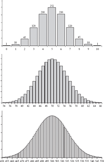
The bars in the graphs above represent the relative magnitudes of the entries in the 10th, 100th, and 1,000th rows of Pascal’s triangle (see chapter 04). The numbers along the horizontal axis indicate to which entry the bar refers. By convention, that labeling begins at 0, rather than 1 (the middle and bottom graphs have been truncated so that the entries whose bars would have negligible height are not shown).

In order to visualize this, have a look at the graph on chapter 07. In this table the data marked by squares concern the guesses made by 300 students, each observing a series of 10 coin flips.²⁶ Along the horizontal axis is plotted the number of correct guesses, from 0 to 10. Along the vertical axis is plotted the number of students who achieved that number of correct guesses. The curve is bell shaped, centered at 5 correct guesses, at which point its height corresponds to about 75 students. The curve falls to about two-thirds of its maximum height, corresponding to about 51 students, about halfway between 3 and 4 correct guesses on the left and between 6 and 7 on the right. A bell curve with this magnitude of standard deviation is typical of a random process such as guessing the result of a coin toss.

The same graph also displays another set of data, marked by circles. That set describes the performance of 300 mutual fund managers. In this case the horizontal axis represents not correct guesses of coin flips but the number of years (out of 10) that a manager performed above the group average. Note the similarity! We’ll get back to this in chapter 9.

A good way to get a feeling for how the normal distribution relates to random error is to consider the process of polling, or sampling. You may recall the poll I described in chapter 5 regarding the popularity of the mayor of Basel. In that city a certain fraction of voters approved of the mayor, and a certain fraction disapproved. For the sake of simplicity we will now assume each was 50 percent. As we saw, there is a chance that those involved in the poll would not reflect exactly this 50/50 split. In fact, if N voters were questioned, the chances that any given number of them would support the mayor are proportional to the numbers on line N of Pascal’s triangle. And so, according to De Moivre’s work, if pollsters poll a large number of voters, the probabilities of different polling results can be described by the normal distribution. In other words about 95 percent of the time the approval rating they observe in their poll will fall within 2 standard deviations of the true rating, 50 percent. Pollsters use the term margin of error to describe this uncertainty. When pollsters tell the media that a poll’s margin of error is plus or minus 5 percent, they mean that if they were to repeat the poll a large number of times, 19 out of 20 (95 percent) of those times the result would be within 5 percent of the correct answer. (Though pollsters rarely point this out, that also means, of course, that about 1 time in 20 the result will be wildly inaccurate.) As a rule of thumb, a sample of 100 yields a margin of error that is too great for most purposes. A sample of 1,000, on the other hand, usually yields a margin of error in the ballpark of 3 percent, which for most purposes suffices.

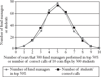
Coin toss guessing compared to stock-picking success

It is important, whenever assessing any kind of survey or poll, to realize that when it is repeated, we should expect the results to vary. For example, if in reality 40 percent of registered voters approve of the way the president is handling his job, it is much more likely that six independent surveys will report numbers like 37, 39, 39, 40, 42, and 42 than it is that all six surveys will agree that the president’s support stands at 40 percent. (Those six numbers are in fact the results of six independent polls gauging the president’s job approval in the first two weeks of September 2006.)²⁷ That’s why, as another rule of thumb, any variation within the margin of error should be ignored. But although The New York Times would not run the headline “Jobs and Wages Increased Modestly at 2 P.M.,” analogous headlines are common in the reporting of political polls. For example, after the Republican National Convention in 2004, CNN ran the headline “Bush Apparently Gets Modest Bounce.”²⁸ The experts at CNN went on to explain that “Bush’s convention bounce appeared to be 2 percentage points…. The percentage of likely voters who said he was their choice for president rose from 50 right before the convention to 52 immediately afterward.” Only later did the reporter remark that the poll’s margin of error was plus or minus 3.5 percentage points, which means that the news flash was essentially meaningless. Apparently the word apparently, in CNN-talk, means “apparently not.”

For many polls a margin of error of more than 5 percent is considered unacceptable, yet in our everyday lives we make judgments based on far fewer data points than that. People don’t get to play 100 years of professional basketball, invest in 100 apartment buildings, or start 100 chocolate-chip-cookie companies. And so when we judge their success at those enterprises, we judge them on just a few data points. Should a football team lavish $50 million to lure a guy coming off a single record-breaking year? How likely is it that the stockbroker who wants your money for a sure thing will repeat her earlier successes? Does the success of the wealthy inventor of sea monkeys mean there is a good chance he’ll succeed with his new ideas of invisible goldfish and instant frogs? (For the record, he didn’t.)²⁹ When we observe a success or a failure, we are observing one data point, a sample from under the bell curve that represents the potentialities that previously existed. We cannot know whether our single observation represents the mean or an outlier, an event to bet on or a rare happening that is not likely to be reproduced. But at a minimum we ought to be aware that a sample point is just a sample point, and rather than accepting it simply as reality, we ought to see it in the context of the standard deviation or the spread of possibilities that produced it. The wine might be rated 91, but that number is meaningless if we have no estimate of the variation that would occur if the identical wine were rated again and again or by someone else. It might help to know, for instance, that a few years back, when both The Penguin Good Australian Wine Guide and On Wine’s Australian Wine Annual reviewed the 1999 vintage of the Mitchelton Blackwood Park Riesling, the Penguin guide gave the wine five stars out of five and named it Penguin Best Wine of the Year, while On Wine rated it at the bottom of all the wines it reviewed, deeming it the worst vintage produced in a decade.³⁰ The normal distribution not only helps us understand such discrepancies, but also has enabled a myriad of statistical applications widely employed today in both science and commerce—for example, whenever a drug company assesses whether the results of a clinical trial are significant, a manufacturer assesses whether a sample of parts accurately reflects the proportion of those that are defective, or a marketer decides whether to act on the results of a research survey.

         

THE RECOGNITION that the normal distribution describes the distribution of measurement error came decades after De Moivre’s work, by that fellow whose name is sometimes attached to the bell curve, the German mathematician Carl Friedrich Gauss. It was while working on the problem of planetary motion that Gauss came to that realization, at least regarding astronomical measurements. Gauss’s “proof,” however, was, by his own later admission, invalid.³¹ Moreover, its far-reaching consequences also eluded him. And so he slipped the law inconspicuously into a section at the end of a book called The Theory of the Motion of Heavenly Bodies Moving about the Sun in Conic Sections. There it may well have died, just another in the growing pile of abandoned proposals for the error law.

It was Laplace who plucked the normal distribution from obscurity. He encountered Gauss’s work in 1810, soon after he had read a memoir to the Académie des Sciences proving a theorem called the central limit theorem, which says that the probability that the sum of a large number of independent random factors will take on any given value is distributed according to the normal distribution. For example, suppose you bake 100 loaves of bread, each time following a recipe that is meant to produce a loaf weighing 1,000 grams. By chance you will sometimes add a bit more or a bit less flour or milk, or a bit more or less moisture may escape in the oven. If in the end each of a myriad of possible causes adds or subtracts a few grams, the central limit theorem says that the weight of your loaves will vary according to the normal distribution. Upon reading Gauss’s work, Laplace immediately realized that he could use it to improve his own and that his work could provide a better argument than Gauss’s to support the notion that the normal distribution is indeed the error law. Laplace rushed to press a short sequel to his memoir on the theorem. Today the central limit theorem and the law of large numbers are the two most famous results of the theory of randomness.

To illustrate how the central limit theorem explains why the normal distribution is the correct error law, let’s reconsider Daniel Bernoulli’s example of the archer. I played the role of the archer one night after a pleasant interlude of wine and adult company, when my younger son, Nicolai, handed me a bow and arrow and dared me to shoot an apple off his head. The arrow had a soft foam tip, but still it seemed reasonable to conduct an analysis of my possible errors and their likelihood. For obvious reasons I was mainly concerned with vertical errors. A simple model of the errors is this: Each random factor—say, a sighting error, the effect of air currents, and so on—would throw my shot vertically off target, either high or low, with equal probability. My total error in aim would then be the sum of my errors. If I was lucky, about half the component errors would deflect the arrow upward and half downward, and my shot would end up right on target. If I was unlucky (or, more to the point, if my son was unlucky), the errors would all fall one way and my aim would be far off, either high or low. The relevant question was, how likely was it that the errors would cancel each other, or that they would add up to their maximum, or that they would take any other value in between? But that was just a Bernoulli process—like tossing coins and asking how likely it is that the tosses will result in a certain number of heads. The answer is described by Pascal’s triangle or, if many trials are involved, by the normal distribution. And that, in this case, is precisely what the central limit theorem tells us. (As it turned out, I missed both apple and son, but did knock over a glass of very nice cabernet.)

By the 1830s most scientists had come to believe that every measurement is a composite, subject to a great number of sources of deviation and hence to the error law. The error law and the central limit theorem thus allowed for a new and deeper understanding of data and their relation to physical reality. In the ensuing century, scholars interested in human society also grasped these ideas and found to their surprise that the variation in human characteristics and behavior often displays the same pattern as the error in measurement. And so they sought to extend the application of the error law from physical science to a new science of human affairs.