CHAPTER 8

The Order in Chaos

IN THE MID-1960S, some ninety years old and in great need of money to live on, a Frenchwoman named Jeanne Calment made a deal with a forty-seven-year-old lawyer: she sold him her apartment for the price of a low monthly subsistence payment with the agreement that the payments would stop upon her death, at which point she would be carried out and he could move in.¹ The lawyer must have known that Ms. Calment had already exceeded the French life expectancy by more than ten years. He may not have been aware of Bayes’s theory, however, nor known that the relevant issue was not whether she should be expected to die in minus ten years but that her life expectancy, given that she had already made it to ninety, was about six more years.² Still, he had to feel comfortable believing that any woman who as a teenager had met Vincent van Gogh in her father’s shop would soon be joining van Gogh in the hereafter. (For the record, she found the artist “dirty, badly dressed, and disagreeable.”)

Ten years later the attorney had presumably found an alternative dwelling, for Jeanne Calment celebrated her 100th birthday in good health. And though her life expectancy was then about two years, she reached her 110th birthday still on the lawyer’s dime. By that point the attorney had turned sixty-seven. But it was another decade before the attorney’s long wait came to an end, and it wasn’t the end he expected. In 1995 the attorney himself died while Jeanne Calment lived on. Her day of reckoning finally came on August 4, 1997, at the age of 122. Her age at death exceeded the lawyer’s age at his death by forty-five years.

Individual life spans—and lives—are unpredictable, but when data are collected from groups and analyzed en masse, regular patterns emerge. Suppose you have driven accident-free for twenty years. Then one fateful afternoon while you’re on vacation in Quebec with your spouse and your in-laws, your mother-in-law yells, “Look out for that moose!” and you swerve into a warning sign that says essentially the same thing. To you the incident would feel like an odd and unique event. But as the need for the sign indicates, in an ensemble of thousands of drivers a certain percentage of drivers can be counted on to encounter a moose. In fact, a statistical ensemble of people acting randomly often displays behavior as consistent and predictable as a group of people pursuing conscious goals. Or as the philosopher Immanuel Kant wrote in 1784, “Each, according to his own inclination follows his own purpose, often in opposition to others; yet each individual and people, as if following some guiding thread, go toward a natural but to each of them unknown goal; all work toward furthering it, even if they would set little store by it if they did know it.”³

According to the Federal Highway Administration, for example, there are about 200 million drivers in the United States.⁴ And according to the National Highway Traffic Safety Administration, in one recent year those drivers drove a total of about 2.86 trillion miles.⁵ That’s about 14,300 miles per driver. Now suppose everyone in the country had decided it would be fun to hit that same total again the following year. Let’s compare two methods that could have been used to achieve that goal. In method 1 the government institutes a rationing system employing one of the National Science Foundation’s supercomputing centers to assign personal mileage targets that meet each of the 200 million motorists’ needs while maintaining the previous annual average of 14,300. In method 2 we tell drivers not to stress out over it and to drive as much or as little as they please with no regard to how far they drove the prior year. If Uncle Billy Bob, who used to walk to work at the liquor store, decides instead to log 100,000 miles as a shotgun wholesaler in West Texas, that’s fine. And if Cousin Jane in Manhattan, who logged most of her mileage circling the block on street-cleaning days in search of a parking space, gets married and moves to New Jersey, we won’t worry about that either. Which method would come closer to the target of 14,300 miles per driver? Method 1 is impossible to test, though our limited experience with gasoline rationing indicates that it probably wouldn’t work very well. Method 2, on the other hand, was actually instituted—that is, the following year, drivers drove as much or as little as they pleased without attempting to hit any quota. How did they do? According to the National Highway Traffic Safety Administration, that year American drivers drove 2.88 trillion miles, or 14,400 miles per person, only 100 miles above target. What’s more, those 200 million drivers also suffered, within less than 200, the same number of fatalities in both years (42,815 versus 42,643).

We associate randomness with disorder. Yet although the lives of 200 million drivers vary unforeseeably, in the aggregate their behavior could hardly have proved more orderly. Analogous regularities can be found if we examine how people vote, buy stocks, marry, are told to get lost, misaddress letters, or sit in traffic on their way to a meeting they didn’t want to go to in the first place—or if we measure the length of their legs, the size of their feet, the width of their buttocks, or the breadth of their beer bellies. As nineteenth-century scientists dug into newly available social data, wherever they looked, the chaos of life seemed to produce quantifiable and predictable patterns. But it was not just the regularities that astonished them. It was also the nature of the variation. Social data, they discovered, often follow the normal distribution.

That the variation in human characteristics and behavior is distributed like the error in an archer’s aim led some nineteenth-century scientists to study the targets toward which the arrows of human existence are aimed. More important, they sought to understand the social and physical causes that sometimes move the target. And so the field of mathematical statistics, developed to aid scientists in data analysis, flourished in a far different realm: the study of the nature of society.

         

STATISTICIANS have been analyzing life’s data at least since the eleventh century, when William the Conqueror commissioned what was, in effect, the first national census. William began his rule in 1035, at age seven, when he succeeded his father as duke of Normandy. As his moniker implies, Duke William II liked to conquer, and in 1066 he invaded England. By Christmas Day he was able to give himself the present of being crowned king. His swift victory left him with a little problem: whom exactly had he conquered, and more important, how much could he tax his new subjects? To answer those questions, he sent inspectors into every part of England to note the size, ownership, and resources of each parcel of land.⁶ To make sure they got it right, he sent a second set of inspectors to duplicate the effort of the first set. Since taxation was based not on population but on land and its usage, the inspectors made a valiant effort to count every ox, cow, and pig but didn’t gather much data about the people who shoveled their droppings. Even if population data had been relevant, in medieval times a statistical survey regarding the most vital statistics about humans—their life spans and diseases—would have been considered inconsistent with the traditional Christian concept of death. According to that doctrine, it was wrong to make death the object of speculation and almost sacrilegious to look for laws governing it. For whether a person died from a lung infection, a stomachache, or a rock whose impact exceeded the compressive strength of his skull, the true cause of his or her death was considered to be simply God’s will. Over the centuries that fatalistic attitude gradually gave way, yielding to an opposing view, according to which, by studying the regularities of nature and society, we are not challenging God’s authority but rather learning about his ways.

A big step in that transformation of views came in the sixteenth century, when the lord mayor of London ordered the compilation of weekly “bills of mortality” to account for the christenings and burials recorded by parish clerks. For decades the bills were compiled sporadically, but in 1603, one of the worst years of the plague, the city instituted a weekly tally. Theorists on the Continent turned up their noses at the data-laden mortality bills as peculiarly English and of little use. But to one peculiar Englishman, a shopkeeper named John Graunt, the tallies told a gripping tale.⁷

Graunt and his friend William Petty have been called the founders of statistics, a field sometimes considered lowbrow by those in pure mathematics owing to its focus on mundane practical issues, and in that sense Graunt in particular makes a fitting founder. For unlike some of the amateurs who developed probability—Cardano the doctor, Fermat the jurist, or Bayes the clergyman—Graunt was a seller of common notions: buttons, thread, needles, and other small items used in a household. But Graunt wasn’t just a button salesman; he was a wealthy button salesman, and his wealth afforded him the leisure to pursue interests having nothing to do with implements for holding garments together. It also enabled him to befriend some of the greatest intellectuals of his day, including Petty.

One inference Graunt gleaned from the mortality bills concerned the number of people who starved to death. In 1665 that number was reported to be 45, only about double the number who died from execution. In contrast, 4,808 were reported to have died from consumption, 1,929 from “spotted fever and purples,” 2,614 from “teeth and worms,” and 68,596 from the plague. Why, when London was “teeming with beggars,” did so few starve? Graunt concluded that the populace must be feeding the hungry. And so he proposed instead that the state provide the food, thereby costing society nothing while ridding seventeenth-century London streets of their equivalent of panhandlers and squeegee men. Graunt also weighed in on the two leading theories of how the plague is spread. One theory held that the illness was transmitted by foul air; the other, that it was transmitted from person to person. Graunt looked at the week-to-week records of deaths and concluded that the fluctuations in the data were too great to be random, as he expected they would be if the person-to-person theory were correct. On the other hand, since weather varies erratically week by week, he considered the fluctuating data to be consistent with the foul-air theory. As it turned out, London was not ready for soup kitchens, and Londoners would have fared better if they had avoided ugly rats rather than foul air, but Graunt’s great discoveries lay not in his conclusions. They lay instead in his realization that statistics can provide insights into the system from which the statistics are derived.

Petty’s work is sometimes considered a harbinger of classical economics.⁸ Believing that the strength of the state depends on, and is reflected by, the number and character of its subjects, Petty employed statistical reasoning to analyze national issues. Typically his analyses were made from the point of view of the sovereign and treated members of society as objects to be manipulated at will. Regarding the plague, he pointed out that money should be spent on prevention because, in saving lives, the realm would preserve part of the considerable investment society made in raising men and women to maturity and therefore would reap a higher return than it would on the most lucrative of alternative investments. Regarding the Irish, Petty was not as charitable. He concluded, for example, that the economic value of an English life was greater than that of an Irish one, so the wealth of the kingdom would be increased if all Irishmen except a few cowherds were forcibly relocated to England. As it happened, Petty owed his own wealth to those same Irish: as a doctor with the invading British army in the 1650s, he had been given the task of assessing the spoils and assessed that he could get away with grabbing a good share for himself, which he did.⁹

If, as Petty believed, the size and growth of a population reflect the quality of its government, then the lack of a good method for measuring the size of a population made the assessment of its government difficult. Graunt’s most famous calculations addressed that issue—in particular the population of London. From the bills of mortality, Graunt knew the number of births. Since he had a rough idea of the fertility rate, he could infer how many women were of childbearing age. That datum allowed him to guess the total number of families and, using his own observations of the mean size of a London family, thereby estimate the city’s population. He came up with 384,000—previously it was believed to be 2 million. Graunt also raised eyebrows by showing that much of the growth of the city was due to immigration from outlying areas, not to the slower method of procreation, and that despite the horrors of the plague, the decrease in population due to even the worst epidemic was always made up within two years. In addition, Graunt is generally credited with publishing the first “life table,” a systematic arrangement of life-expectancy data that today is widely employed by organizations—from life insurance companies to the World Health Organization—that are interested in knowing how long people live. A life table displays how many people, in a group of 100, can be expected to survive to any given age. To Graunt’s data (the column in the table below labeled “London, 1662”), I’ve added columns exhibiting the same data for a few countries today.¹⁰

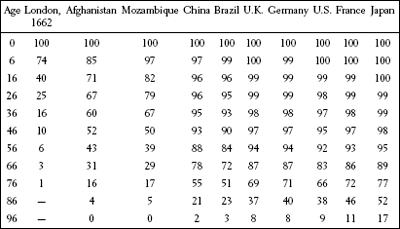
Graunt’s life table extended

In 1662, Graunt published his analyses in Natural and Political Observations…upon the Bills of Mortality. The book met with acclaim. A year later Graunt was elected to the Royal Society. Then, in 1666, the Great Fire of London, which burned down a large part of the city, destroyed his business. To add insult to injury, he was accused of helping to cause the destruction by giving instructions to halt the water supply just before the fire started. In truth he had no affiliation with the water company until after the fire. Still, after that episode, Graunt’s name disappeared from the books of the Royal Society. Graunt died of jaundice a few years later.

Largely because of Graunt’s work, in 1667 the French fell in line with the British and revised their legal code to enable surveys like the bills of mortality. Other European countries followed suit. By the nineteenth century, statisticians all over Europe were up to their elbows in government records such as census data—“an avalanche of numbers.”¹¹ Graunt’s legacy was to demonstrate that inferences about a population as a whole could be made by carefully examining a limited sample of data. But though Graunt and others made valiant efforts to learn from the data through the application of simple logic, most of the data’s secrets awaited the development of the tools created by Gauss, Laplace, and others in the nineteenth and early twentieth centuries.

         

THE TERM statistics entered the English language from the German word Statistik through a 1770 translation of the book Bielfield’s Elementary Universal Education, which stated that “the science that is called statistics teaches us what is the political arrangement of all the modern states in the known world.”¹² By 1828 the subject had evolved such that Noah Webster’s American Dictionary defined statistics as “a collection of facts respecting the state of society, the condition of the people in a nation or country, their health, longevity, domestic economy, arts, property and political strength, the state of their country, &c.”¹³ The field had embraced the methods of Laplace, who had sought to extend his mathematical analysis from planets and stars to issues of everyday life.

The normal distribution describes the manner in which many phenomena vary around a central value that represents their most probable outcome; in his Essai philosophique sur les probabilités, Laplace argued that this new mathematics could be employed to assess legal testimony, predict marriage rates, calculate insurance premiums. But by the final edition of that work, Laplace was in his sixties, and so it fell to a younger man to develop his ideas. That man was Adolphe Quételet, born in Ghent, Flanders, on February 22, 1796.¹⁴

Quételet did not enter his studies spurred by a keen interest in the workings of society. His dissertation, which in 1819 earned him the first doctorate in science awarded by the new university in Ghent, was on the theory of conic sections, a topic in geometry. His interest then turned to astronomy, and around 1820 he became active in a movement to found a new observatory in Brussels, where he had taken a position. An ambitious man, Quételet apparently saw the observatory as a step toward establishing a scientific empire. It was an audacious move, not least because he knew relatively little about astronomy and virtually nothing about running an observatory. But he must have been persuasive, because not only did his observatory receive funding, but he personally received a grant to travel to Paris for several months to remedy the deficiencies in his knowledge. It proved a sound investment, for Quételet’s Royal Observatory of Belgium is still in existence today.

In Paris, Quételet was affected in his own way by the disorder of life, and it pulled him in a completely different direction. His romance with statistics began when he made the acquaintance of several great French mathematicians, including Laplace and Joseph Fourier, and studied statistics and probability with Fourier. In the end, though he learned how to run an observatory, he fell in love with a different pursuit, the idea of applying the mathematical tools of astronomy to social data.

When Quételet returned to Brussels, he began to collect and analyze demographic data, soon focusing on records of criminal activity that the French government began to publish in 1827. In Sur l’homme et le développement de ses facultés, a two-volume work he published in 1835, Quételet printed a table of annual murders reported in France from 1826 to 1831. The number of murders, he noted, was relatively constant, as was the proportion of murders committed each year with guns, swords, knives, canes, stones, instruments for cutting and stabbing, kicks and punches, strangulation, drowning, and fire.¹⁵ Quételet also analyzed mortality according to age, geography, season, and profession, as well as in hospitals and prisons. He studied statistics on drunkenness, insanity, and crime. And he discovered statistical regularities describing suicide by hanging in Paris and the number of marriages between sixty-something women and twenty-something men in Belgium.

Statisticians had conducted such studies before, but Quételet did something more with the data: he went beyond examining the average to scrutinizing the manner in which the data strayed from its average. Wherever he looked, Quételet found the normal distribution: in the propensities to crime, marriage, and suicide and in the height of American Indians and the chest measurements of Scottish soldiers (he came upon a sample of 5,738 chest measurements in an old issue of the Edinburgh Medical and Surgical Journal). In the height of 100,000 young Frenchmen called up for the draft he also found meaning in a deviation from the normal distribution. In that data, when the number of conscripts was plotted against their height, the bell-shaped curve was distorted: too few prospects were just above five feet two and a compensating surplus was just below that height. Quételet argued that the difference—about 2,200 extra “short men”—was due to fraud or, you might say friendly fudging, as those below five feet two were excused from service.

Decades later the great French mathematician Jules-Henri Poincaré employed Quételet’s method to nab a baker who was shortchanging his customers. At first, Poincaré, who made a habit of picking up a loaf of bread each day, noticed after weighing his loaves that they averaged about 950 grams instead of the 1,000 grams advertised. He complained to the authorities and afterward received bigger loaves. Still he had a hunch that something about his bread wasn’t kosher. And so with the patience only a famous—or at least tenured—scholar can afford, he carefully weighed his bread every day for the next year. Though his bread now averaged closer to 1,000 grams, if the baker had been honestly handing him random loaves, the number of loaves heavier and lighter than the mean should have—as I mentioned in chapter 7—diminished following the bell-shaped pattern of the error law. Instead, Poincaré found that there were too few light loaves and a surplus of heavy ones. He concluded that the baker had not ceased baking underweight loaves but instead was seeking to placate him by always giving him the largest loaf he had on hand. The police again visited the cheating baker, who was reportedly appropriately astonished and presumably agreed to change his ways.¹⁶

Quételet had stumbled on a useful discovery: the patterns of randomness are so reliable that in certain social data their violation can be taken as evidence of wrongdoing. Today such analyses are applied to reams of data too large to have been analyzed in Quételet’s time. In recent years, in fact, such statistical sleuthing has become popular, creating a new field, called forensic economics, perhaps the most famous example of which is the statistical study suggesting that companies were backdating their stock option grants. The idea is simple: companies grant stock options—the right to buy shares later at the price of the stock on the date of the grant—as an incentive for executives to improve their firms’ share prices. If the grants are backdated to times when the shares were especially low, the executives’ profits will be correspondingly high. A clever idea, but when done in secret it violates securities laws. It also leaves a statistical fingerprint, which has led to the investigation of such practices at about a dozen major companies.¹⁷ In a less publicized example, Justin Wolfers, an economist at the Wharton School, found evidence of fraud in the results of about 70,000 college basketball games.¹⁸

Wolfers discovered the anomaly by comparing Las Vegas bookmakers’ point spreads to the games’ actual outcomes. When one team is favored, the bookmakers offer point spreads in order to attract a roughly even number of bets on both competitors. For instance, suppose the basketball team at Caltech is considered better than the team at UCLA (for college basketball fans, yes, this was actually true in the 1950s). Rather than assigning lopsided odds, bookies could instead offer an even bet on the game but pay out on a Caltech bet only if their team beat UCLA by, say, 13 or more points.

Though such point spreads are set by the bookies, they are really fixed by the mass of bettors because the bookies adjust them to balance the demand. (Bookies make their money on fees and seek to have an equal amount of money bet on each side so that they can’t lose, whatever the outcome.) To measure how well bettors assess two teams, economists use a number called the forecast error, which is the difference between the favored team’s margin of victory and the point spread determined by the marketplace. It may come as no surprise that forecast error, being a type of error, is distributed according to the normal distribution. Wolfers found that its mean is 0, meaning that the point spreads don’t tend to either overrate or underrate teams, and its standard deviation is 10.9 points, meaning that about two thirds of the time the point spread is within 10.9 points of the margin of victory. (In a study of professional football games, a similar result was found, with a mean of 0 and a standard deviation of 13.9 points.)¹⁹

When Wolfers examined the subset of games that involved heavy favorites, he found something astonishing: there were too few games in which the heavy favorite won by a little more than the point spread and an inexplicable surplus of games in which the favorite won by just less. This was again Quételet’s anomaly. Wolfers’s conclusion, like Quételet’s and Poincaré’s, was fraud. His analysis went like this: it is hard for even a top player to ensure that his team will beat a point spread, but if the team is a heavy favorite, a player, without endangering his team’s chance of victory, can slack off enough to ensure that the team does not beat the spread. And so if unscrupulous bettors wanted to fix games without asking players to risk losing, the result would be just the distortions Wolfers found. Does Wolfers’s work prove that in some percentage of college basketball games, players are taking bribes to shave points? No, but as Wolfers says, “You shouldn’t have what’s happening on the court reflecting what’s happening in Las Vegas.” And it is interesting to note that in a recent poll by the National Collegiate Athletic Association, 1.5 percent of players admitted knowing a teammate “who took money for playing poorly.”²⁰

         

QUÉTELET DID NOT PURSUE the forensic applications of his ideas. He had bigger plans: to employ the normal distribution in order to illuminate the nature of people and society. If you made 1,000 copies of a statue, he wrote, those copies would vary due to errors of measurement and workmanship, and that variation would be governed by the error law. If the variation in people’s physical traits follows the same law, he reasoned, it must be because we, too, are imperfect replicas of a prototype. Quételet called that prototype l’homme moyen, the average man. He felt that a template existed for human behavior too. The manager of a large department store may not know whether the spacey new cashier will pocket that half-ounce bottle of Chanel Allure she was sniffing, but he can count on the prediction that in the retail business, inventory loss runs pretty steadily from year to year at about 1.6 percent and that consistently about 45 percent to 48 percent of it is due to employee theft.²¹ Crime, Quételet wrote, is “like a budget that is paid with frightening regularity.”²²

Quételet recognized that l’homme moyen would be different for different cultures and that it could change with changing social conditions. In fact, it is the study of those changes and their causes that was Quételet’s greatest ambition. “Man is born, grows up, and dies according to certain laws,” he wrote, and those laws “have never been studied.”²³ Newton became the father of modern physics by recognizing and formulating a set of universal laws. Modeling himself after Newton, Quételet desired to create a new “social physics” describing the laws of human behavior. In Quételet’s analogy, just as an object, if undisturbed, continues in its state of motion, so the mass behavior of people, if social conditions remain unchanged, remains constant. And just as Newton described how physical forces deflect an object from its straight path, so Quételet sought laws of human behavior describing how social forces transform the characteristics of society. For example, Quételet thought that vast inequalities of wealth and great fluctuations in prices were responsible for crime and social unrest and that a steady level of crime represented a state of equilibrium, which would change with changes in the underlying causes. A vivid example of such a change in social equilibrium occurred in the months after the attacks of September 11, 2001, when travelers, afraid to take airplanes, suddenly switched to cars. Their fear translated into about 1,000 more highway fatalities in that period than in the same period the year before—hidden casualties of the September 11 attack.²⁴

But to believe that a social physics exists is one thing, and to define one is another. In a true science, Quételet realized, theories could be explored by placing people in a great number of experimental situations and measuring their behavior. Since that is not possible, he concluded that social science is more like astronomy than physics, with insights deduced from passive observation. And so, seeking to uncover the laws of social physics, he studied the temporal and cultural variation in l’homme moyen.

Quételet’s ideas were well received, especially in France and Great Britain. One physiologist even collected urine from a railroad-station urinal frequented by people of many nationalities in order to determine the properties of the “average European urine.”²⁵ In Britain, Quételet’s most enthusiastic disciple was a wealthy chess player and historian named Henry Thomas Buckle, best known for an ambitious multivolume book called History of Civilization in England. Unfortunately, in 1861, when he was forty, Buckle caught typhus while traveling in Damascus. Offered the services of a local physician, he refused because the man was French, and so he died. Buckle hadn’t finished his treatise. But he did complete the initial two volumes, the first of which presented history from a statistical point of view. It was based on the work of Quételet and was an instant success. Read throughout Europe, it was translated into French, German, and Russian. Darwin read it; Alfred Russel Wallace read it; Dostoyevsky read it twice.²⁶

Despite the book’s popularity, the verdict of history is that Quételet’s mathematics proved more sensible than his social physics. For one thing, not all that happens in society, especially in the financial realm, is governed by the normal distribution. For example, if film revenue were normally distributed, most films would earn near some average amount, and two-thirds of all film revenue would fall within a standard deviation of that number. But in the film business, 20 percent of the movies bring in 80 percent of the revenue. Such hit-driven businesses, though thoroughly unpredictable, follow a far different distribution, one for which the concepts of mean and standard deviation have no meaning because there is no “typical” performance, and megahit outliers, which in an ordinary business might occur only once every few centuries, happen every few years.²⁷

More important than his ignoring other probability distributions, though, is Quételet’s failure to make much progress in uncovering the laws and forces he sought. So in the end his direct impact on the social sciences proved modest, yet his legacy is both undeniable and far-reaching. It lies not in the social sciences but in the “hard” sciences, where his approach to understanding the order in large numbers of random events inspired many scholars and spawned revolutionary work that transformed the manner of thinking in both biology and physics.

         

IT WAS CHARLES DARWIN’S FIRST COUSIN who introduced statistical thinking to biology. A man of leisure, Francis Galton had entered Trinity College, Cambridge, in 1840.²⁸ He first studied medicine but then followed Darwin’s advice and changed his field to mathematics. He was twenty-two when his father died and he inherited a substantial sum. Never needing to work for a living, he became an amateur scientist. His obsession was measurement. He measured the size of people’s heads, noses, and limbs, the number of times people fidgeted while listening to lectures, and the degree of attractiveness of girls he passed on the street (London girls scored highest; Aberdeen, lowest). He measured the characteristics of people’s fingerprints, an endeavor that led to the adoption of fingerprint identification by Scotland Yard in 1901. He even measured the life spans of sovereigns and clergymen, which, being similar to the life spans of people in other professions, led him to conclude that prayer brought no benefit.

In his 1869 book, Hereditary Genius, Galton wrote that the fraction of the population in any given range of heights must be nearly uniform over time and that the normal distribution governs height and every other physical feature: circumference of the head, size of the brain, weight of the gray matter, number of brain fibers, and so on. But Galton didn’t stop there. He believed that human character, too, is determined by heredity and, like people’s physical features, obeys in some manner the normal distribution. And so, according to Galton, men are not “of equal value, as social units, equally capable of voting, and the rest.”²⁹ Instead, he asserted, about 250 out of every 1 million men inherit exceptional ability in some area and as a result become eminent in their field. (As, in his day, women did not generally work, he did not make a similar analysis of them.) Galton founded a new field of study based on those ideas, calling it eugenics, from the Greek words eu (good) and genos (birth). Over the years, eugenics has meant many different things to many different people. The term and some of his ideas were adopted by the Nazis, but there is no evidence that Galton would have approved of the Germans’ murderous schemes. His hope, rather, was to find a way to improve the condition of humankind through selective breeding.

Much of chapter 9 is devoted to understanding the reasons Galton’s simple cause-and-effect interpretation of success is so seductive. But we’ll see in chapter 10 that because of the myriad of foreseeable and chance obstacles that must be overcome to complete a task of any complexity, the connection between ability and accomplishment is far less direct than anything that can possibly be explained by Galton’s ideas. In fact, in recent years psychologists have found that the ability to persist in the face of obstacles is at least as important a factor in success as talent.³⁰ That’s why experts often speak of the “ten-year rule,” meaning that it takes at least a decade of hard work, practice, and striving to become highly successful in most endeavors. It might seem daunting to think that effort and chance, as much as innate talent, are what counts. But I find it encouraging because, while our genetic makeup is out of our control, our degree of effort is up to us. And the effects of chance, too, can be controlled to the extent that by committing ourselves to repeated attempts, we can increase our odds of success.

Whatever the pros and cons of eugenics, Galton’s studies of inheritance led him to discover two mathematical concepts that are central to modern statistics. One came to him in 1875, after he distributed packets of sweet pea pods to seven friends. Each friend received seeds of uniform size and weight and returned to Galton the seeds of the successive generations. On measuring them, Galton noticed that the median diameter of the offspring of large seeds was less than that of the parents, whereas the median diameter of the offspring of small seeds was greater than that of the parents. Later, employing data he obtained from a laboratory he had set up in London, he noticed the same effect in the height of human parents and children. He dubbed the phenomenon—that in linked measurements, if one measured quantity is far from its mean, the other will be closer to its mean—regression toward the mean.

Galton soon realized that processes that did not exhibit regression toward the mean would eventually go out of control. For example, suppose the sons of tall fathers would on average be as tall as their fathers. Since heights vary, some sons would be taller. Now imagine the next generation, and suppose the sons of the taller sons, grandsons of the original men, were also on average as tall as their fathers. Some of them, too, would have to be taller than their fathers. In this way, as generation followed generation, the tallest humans would be ever taller. Because of regression toward the mean, that does not happen. The same can be said of innate intelligence, artistic talent, or the ability to hit a golf ball. And so very tall parents should not expect their children to be as tall, very brilliant parents should not expect their children to be as brilliant, and the Picassos and Tiger Woodses of this world should not expect their children to match their accomplishments. On the other hand, very short parents can expect taller offspring, and those of us who are not brilliant or can’t paint have reasonable hope that our deficiencies will be improved upon in the next generation.

At his laboratory, Galton attracted subjects through advertisements and then subjected them to a series of measurements of height, weight, even the dimensions of certain bones. His goal was to find a method for predicting the measurements of children based on those of their parents. One of Galton’s plots showed parents’ heights versus the heights of their offspring. If, say, those heights were always equal, the graph would be a neat line rising at 45 degrees. If that relationship held on average but individual data points varied, then the data would show some scatter above and below that line. Galton’s graphs thus exhibited visually not just the general relationship between the heights of parent and offspring but also the degree to which the relationship holds. That was Galton’s other major contribution to statistics: defining a mathematical index describing the consistency of such relationships. He called it the coefficient of correlation.

The coefficient of correlation is a number between -1 and 1; if it is near ± 1, it indicates that two variables are linearly related; a coefficient of 0 means there is no relation. For example, if data revealed that by eating the latest McDonald’s 1,000-calorie meal once a week, people gained 10 pounds a year and by eating it twice a week they gained 20 pounds, and so on, the correlation coefficient would be 1. If for some reason everyone were to instead lose those amounts of weight, the correlation coefficient would be -1. And if the weight gain and loss were all over the map and didn’t depend on meal consumption, the coefficient would be 0. Today correlation coefficients are among the most widely employed concepts in statistics. They are used to assess such relationships as those between the number of cigarettes smoked and the incidence of cancer, the distance of stars from Earth and the speed with which they are moving away from our planet, and the scores students achieve on standardized tests and the income of the students’ families.

Galton’s work was significant not just for its direct importance but because it inspired much of the statistical work done in the decades that followed, in which the field of statistics grew rapidly and matured. One of the most important of these advances was made by Karl Pearson, a disciple of Galton’s. Earlier in this chapter, I mentioned many types of data that are distributed according to the normal distribution. But with a finite set of data the fit is never perfect. In the early days of statistics, scientists sometimes determined whether data were normally distributed simply by graphing them and observing the shape of the resulting curve. But how do you quantify the accuracy of the fit? Pearson invented a method, called the chi-square test, by which you can determine whether a set of data actually conforms to the distribution you believe it conforms to. He demonstrated his test in Monte Carlo in July 1892, performing a kind of rigorous repeat of Jagger’s work.³¹ In Pearson’s test, as in Jagger’s, the numbers that came up on a roulette wheel did not follow the distribution they would have followed if the wheel had produced random results. In another test, Pearson examined how many 5s and 6s came up in 26,306 tosses of twelve dice. He found that the distribution was not one you’d see in a chance experiment with fair dice—that is, in an experiment in which the probability of a 5 or a 6 on one roll were 1 in 3, or 0.3333. But it was consistent if the probability of a 5 or a 6 were 0.3377—that is, if the dice were skewed. In the case of the roulette wheel the game may have been rigged, but the dice were probably biased owing to variations in manufacturing, which my friend Moshe emphasized are always present.

Today chi-square tests are widely employed. Suppose, for instance, that instead of testing dice, you wish to test three cereal boxes for their consumer appeal. If consumers have no preference, you would expect about 1 in 3 of those polled to vote for each box. As we’ve seen, the actual results will rarely be distributed so evenly. Employing the chi-square test, you can determine how likely it is that the winning box received more votes due to consumer preference rather than to chance. Similarly, suppose researchers at a pharmaceutical company perform an experiment in which they test two treatments used in preventing acute transplant rejection. They can use a chi-square test to determine whether there is a statistically significant difference between the results. Or suppose that before opening a new outlet, the CFO of a rental car company expects that 25 percent of the company’s customers will request subcompact cars, 50 percent will want compacts, and 12.5 percent each will ask for cars in the midsize and “other” categories. When the data begin to come in, a chi-square test can help the CFO quickly decide whether his assumption was correct or the new site is atypical and the company would do well to alter the mix.

Through Galton, Quételet’s work infused the biological sciences. But Quételet also helped spur a revolution in the physical sciences: both James Clerk Maxwell and Ludwig Boltzmann, two of the founders of statistical physics, drew inspiration from Quételet’s theories. (Like Darwin and Dostoyevsky, they read of them in Buckle’s book.) After all, if the chests of 5,738 Scottish soldiers distribute themselves nicely along the curve of the normal distribution and the average yearly mileage of 200 million drivers can vary by as little as 100 miles from year to year, it doesn’t take an Einstein to guess that the 10 septillion or so molecules in a liter of gas might exhibit some interesting regularities. But actually it did take an Einstein to finally convince the scientific world of the need for that new approach to physics. Albert Einstein did it in 1905, the same year in which he published his first work on relativity. And though hardly known in popular culture, Einstein’s 1905 paper on statistical physics proved equally revolutionary. In the scientific literature, in fact, it would become his most cited work.³²

         

EINSTEIN’S 1905 WORK on statistical physics was aimed at explaining a phenomenon called Brownian motion. The process was named for Robert Brown, botanist, world expert in microscopy, and the person credited with writing the first clear description of the cell nucleus. Brown’s goal in life, pursued with relentless energy, was to discover through his observations the source of the life force, a mysterious influence believed in his day to endow something with the property of being alive. In that quest, Brown was doomed to failure, but one day in June 1827, he thought he had succeeded.

Peering through his lens, Brown noted that the granules inside the pollen grains he was observing seemed to be moving.³³ Though a source of life, pollen is not itself a living being. Yet as long as Brown stared, the movement never ceased, as if the granules possessed some mysterious energy. This was not intentioned movement; it seemed, in fact, to be completely random. With great excitement, Brown concluded at first that he had bagged his quarry, for what could this energy be but the energy that powers life itself?

In a string of experiments he performed assiduously over the next month, Brown observed the same kind of movement when suspending in water, and sometimes in gin, as wide a variety of organic particles as he could get his hands on: decomposing fibers of veal, spider’s web “blackened with London dust,” even his own mucus. Then, in a deathblow to his wishful interpretation of the discovery, Brown also observed the motion when looking at inorganic particles—of asbestos, copper, bismuth, antimony, and manganese. He knew then that the movement he was observing was unrelated to the issue of life. The true cause of Brownian motion would prove to be the same force that compelled the regularities in human behavior that Quételet had noted—not a physical force but an apparent force arising from the patterns of randomness. Unfortunately, Brown did not live to see this explanation of the phenomenon he observed.

The groundwork for the understanding of Brownian motion was laid in the decades that followed Brown’s work, by Boltzmann, Maxwell, and others. Inspired by Quételet, they created the new field of statistical physics, employing the mathematical edifice of probability and statistics to explain how the properties of fluids arise from the movement of the (then hypothetical) atoms that make them up. Their ideas did not catch on for several more decades, however. Some scientists had mathematical issues with the theory. Others objected because at the time no one had ever seen an atom and no one believed anyone ever would. But most physicists are practical, and so the most important roadblock to acceptance was that although the theory reproduced some laws that were known, it made few new predictions. And so matters stood until 1905, when long after Maxwell was dead and shortly before a despondent Boltzmann would commit suicide, Einstein employed the nascent theory to explain in great numerical detail the precise mechanism of Brownian motion.³⁴ The necessity of a statistical approach to physics would never again be in doubt, and the idea that matter is made of atoms and molecules would prove to be the basis of most modern technology and one of the most important ideas in the history of physics.

The random motion of molecules in a fluid can be viewed, as we’ll note in chapter 10, as a metaphor for our own paths through life, and so it is worthwhile to take a little time to give Einstein’s work a closer look. According to the atomic picture, the fundamental motion of water molecules is chaotic. The molecules fly first this way, then that, moving in a straight line only until deflected by an encounter with one of their sisters. As mentioned in the Prologue, this type of path—in which at various points the direction changes randomly—is often called a drunkard’s walk, for reasons obvious to anyone who has ever enjoyed a few too many martinis (more sober mathematicians and scientists sometimes call it a random walk). If particles that float in a liquid are, as atomic theory predicts, constantly and randomly bombarded by the molecules of the liquid, one might expect them to jiggle this way and that owing to the collisions. But there are two problems with that picture of Brownian motion: first, the molecules are far too light to budge the visible floating particles; second, molecular collisions occur far more frequently than the observed jiggles. Part of Einstein’s genius was to realize that those two problems cancel each other out: though the collisions occur very frequently, because the molecules are so light, those frequent isolated collisions have no visible effect. It is only when pure luck occasionally leads to a lopsided preponderance of hits from some particular direction—the molecular analogue of Roger Maris’s record year in baseball—that a noticeable jiggle occurs. When Einstein did the math, he found that despite the chaos on the microscopic level, there was a predictable relationship between factors such as the size, number, and speed of the molecules and the observable frequency and magnitude of the jiggling. Einstein had, for the first time, connected new and measurable consequences to statistical physics. That might sound like a largely technical achievement, but on the contrary, it represented the triumph of a great principle: that much of the order we perceive in nature belies an invisible underlying disorder and hence can be understood only through the rules of randomness. As Einstein wrote, “It is a magnificent feeling to recognize the unity of a complex of phenomena which appear to be things quite apart from the direct visible truth.”³⁵

In Einstein’s mathematical analysis the normal distribution again played a central role, reaching a new place of glory in the history of science. The drunkard’s walk, too, became established as one of the most fundamental—and soon one of the most studied—processes in nature. For as scientists in all fields began to accept the statistical approach as legitimate, they recognized the thumbprints of the drunkard’s walk in virtually all areas of study—in the foraging of mosquitoes through cleared African jungle, in the chemistry of nylon, in the formation of plastics, in the motion of free quantum particles, in the movement of stock prices, even in the evolution of intelligence over eons of time. We’ll examine the effects of randomness on our own paths through life in chapter 10. But as we’re about to see, though in random variation there are orderly patterns, patterns are not always meaningful. And as important as it is to recognize the meaning when it is there, it is equally important not to extract meaning when it is not there. Avoiding the illusion of meaning in random patterns is a difficult task. It is the subject of the following chapter.