1

Introduction

In this chapter, we present some basic concepts and ideas of number theory, computation theory, computational number theory, and modern (number-theoretic) cryptography. More specifically, we shall try to answer the following typical questions in the field:

• What is number theory?
• What is computation theory?
• What is computational number theory?
• What is modern (number-theoretic) cryptography?

1.1 What is Number Theory?

Number theory is concerned mainly with the study of the properties (e.g., the divisibility) of the integers

particularly the positive integers

For example, in divisibility theory, all positive integers can be classified into three classes:

1. Unit: 1.

2. Prime numbers: 2, 3, 5, 7, 11, 13, 17, 19,....

3. Composite numbers: 4, 6, 8, 9, 10, 12, 14, 15,....

Recall that a positive integer n>1 is called a prime number, if its only divisors are 1 and n, otherwise, it is a composite number. 1 is neither prime number nor composite number. Prime numbers play a central role in number theory, as any positive integer n>1 can be written uniquely into the following standard prime factorization form:

(1.1)

where p1<p2<...<pk are primes and positive integers. Although prime numbers have been studied for more than 2000 years, there are still many open problems about their distribution. Let us investigate some of the most interesting problems about prime numbers.

1. The distribution of prime numbers.

Euclid proved 2000 years ago in his Elements that there were infinitely many prime numbers. That is, the sequence of prime numbers

is endless. For example, 2, 3, 5 are the first three prime numbers, whereas 243112609−1 is the largest prime number to date, it has 12978189 digits and was found on 23 August 2008. Let denote the prime numbers up to x (Table 1.1 gives some values of for some large x), then Euclid’s theorem of infinitude of primes actually says that

A much better result about the distribution of prime numbers is the Prime Number theorem, stating that

(1.2)

In other words,

(1.3)

Note that the log  is the natural logarithm loge (normally denoted by ln ), where e = 2.7182818.... However, if the Riemann Hypothesis [3] is true, then there is a refinement of the Prime Number theorem

(1.4)

to the effect that

(1.5)

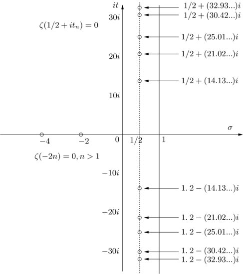
Of course we do not know if the Riemann Hypothesis is true. Whether or not the Riemann Hypothesis is true is one of the most important open problems in mathematics, and in fact it is one of the seven Millennium Prize Problems proposed by the Clay Mathematics Institute in Boston in 2000, each with a one million US dollars prize [4]. The Riemann hypothesis states that all the nontrivial (complex) zeros of the function

(1.6)

lying in the critical strip 0<Re(s)<1 must lie on the critical line , that is, , where denotes a nontrivial zero of . Riemann calculated the first five nontrivial zeros of and found that they all lie on the critical line (see Figure 1.1), he then conjectured that all the nontrivial zeros of are on the critical line.

2. The distribution of twin prime numbers.

Twin prime numbers are of the form , where both numbers are prime. For example, (3, 5), (5, 7), (11, 13) are the first three smallest twin prime pairs, whereas the largest twin primes so far are , discovered in August 2009, both numbers having 100355 digits. Table 1.2 gives 10 large twin prime pairs. Let be the number of twin primes up to x (Table 1.3 gives some values of for different x), then the twin prime conjecture states that

If the probability of a random integer x and the integer x+2 being prime were statistically independent, then it would follow from the prime number theorem that

(1.7)

or more precisely,

(1.8)

with

(1.9)

As these probabilities are not independent, so Hardy and Littlewood conjectured that

(1.10)

The infinite product in the above formula is the twin prime constant; this constant was estimated to be approximately 0.6601618158.... Using very complicated arguments based on sieve methods, in his work on the Goldbach conjecture, the Chinese mathematician Chen showed that there are infinitely many pairs of integers (n, n+2), with n prime and n+2 a product of at most two primes. The famous Goldbach conjecture states that every even number greater than 4 is the sum of two odd prime numbers. It was conjectured by Goldbach in a letter to Euler in 1742. It remains unsolved to this day. The best result for this conjecture is due to Chen, who announced it in 1966, but the full proof was not given until 1973 due to the chaotic Cultural Revolution, that every sufficiently large even number is the sum of one prime number and the product of at most two prime numbers, that is, E=p1+p2p3, where E is a sufficiently large even number and p1, p2, p3 are prime numbers. As a consequence, there are infinitely many such twin numbers (p1, p1+2=p2p3). Extensions relating to the twin prime numbers have also been considered. For example, are there infinitely many triplet primes (p, q, r) with q=p+2 and r=p+6? The first five triplets of this form are as follows: (5, 7, 11), (11, 13, 17), (17, 19, 23), (41, 43, 47), (101, 103, 107). The triplet prime problem is much harder than the twin prime problem. It is amusing to note that there is only one triplet prime (p, q, r) with q=p+2 and r=p+4. That is, (3, 5, 7). The Riemann Hypothesis, the Twin Prime Problem, and the Goldbach conjecture form the famous Hilbert’s 8th Problem.

3. The distribution of arithmetic progressions of prime numbers.

An arithmetic progression of prime numbers is defined to be the sequence of primes satisfying:

(1.11)

where p is the first term, d the common difference, and p+(k−1)d the last term of the sequence. For example, the following are some sequences of the arithmetic progression of primes:

The longest arithmetic progression of primes is the following sequence with 23 terms: 56211383760397 + k.44546738095860 with k=0, 1, ... , 22. Thanks to Green and Tao who proved in 2007 that there are arbitrary long arithmetic progressions of primes (i.e., k can be any arbitrary large natural number), which enabled, among others, Tao to receive a Field Prize in 2006, the equivalent to a Nobel Prize for Mathematics. However, their result is not about consecutive primes; we still do not know if there are arbitrary long arithmetic progressions of consecutive primes, although Chowa proved in 1944 that there exists an infinity of three consecutive primes of arithmetic progressions. Note that an arithmetic progression of consecutive primes is a sequence of consecutive primes in the progression. In 1967, Jones, Lal, and Blundon found an arithmetic progression of five consecutive primes 1010+24493+30k with k=0, 1, 2, 3, 4. In the same year, Lander and Parkin discovered six in an arithmetic progression 121174811+30k with k=0, 1, 2, 3, 4, 5. The longest arithmetic progression of consecutive primes, discovered by Manfred Toplic in 1998, is 507618446770482.193# + x77 + 210k, where 193# is the product of all primes 193, that is, 193# = 2. 3. 5. 7... 193, x77 is a 77-digit number 54538241683887582668189703590110659057865934764604873840781923513421103495579 and k=0, 1, 2, ..., 9.

Figure 1.1 Riemann hypothesis

Table 1.1 for some large x

x
1015	29844570422669
1016	279238341033925
1017	2623557157654233
1018	24739954287740860
1019	234057667276344607
1020	2220819602560918840
1021	21127269486018731928
1022	201467286689315906290
1023	1925320391606803968923
1024	18435599767349200867866

Table 1.2 Ten large twin prime pairs

Table 1.3 for some large values

Table 1.4 The 47 known Mersenne primes Mp=2p−1

It should be noted that problems in number theory are easy to state, because they are mainly concerned with integers with which we are very familiar, but often very hard to solve!

Problems for Section 1.1

1. Show that there are infinitely many prime numbers.

2. Prove or disprove there are infinitely many twin prime numbers.

3. Are there infinitely many triple prime numbers of the form p, p+2, p+4, where p, p+2, p+4 are all prime numbers? For example, 3, 5, 7 are such triple prime numbers.

4. Are there infinitely many triple prime numbers of the form p, p+2, p+6, where p, p+2, p+6 are all prime numbers? For example, 5, 7, 11 are such triple prime numbers.

5. (Prime Number Theorem) Show that

6. The Riemann -function is defined as follows:

where is a complex number. Riemann conjectured that all zeroes of in the critical strip must lie on the critical line . That is,

Prove or disprove the Riemann Hypothesis.

7. Andrew Beal in 1993 conjectured that the equation xa+yb=zc has no positive integer solutions in x, y, z, a, b, c, where a,b,c 3 and gcd(x,y)=(y,z)=(x,z)=1. Beal has offered $100 000 for a proof or a disproof of this conjecture.

8. Prove or disprove the Goldbach conjecture that any even number greater than 6 is the sum of two odd prime numbers.

9. A positive integer n is perfect if σ (n) =2n, where σ (n) is the sum of all divisors of n. For example, 6 is perfect since σ (6)= 1+2+3+6= 2. 6 = 12. Show n is perfect if and only if n=2p−1(2p−1), where 2p−1 is a Mersenne prime.

10. All known perfect numbers are even perfect. Recent research shows that if there exists an odd perfect number, it must be greater than 10300 and must have at least 29 prime factors (not necessarily distinct). Prove or disprove that there exists at least one odd perfect number.

11. Show that there are arbitrary long arithmetic progressions of prime numbers

where p is the first term, d the common difference, and p+(k−1)d the last term of the sequence, and furthermore, all the terms in the sequence are prime numbers and k can be any arbitrary large positive integer.

12. Prove or disprove that there are arbitrary long arithmetic progressions of consecutive prime numbers.

1.2 What is Computation Theory?

Computation theory, or the theory of computation, is a branch that deals with whether and how efficiently problems can be solved on a model of computation, using an algorithm. It may be divided into two main branches: Computability theory and computational complexity theory. Generally speaking, computability theory deals with what a computer can or cannot do theoretically (i.e., without any restrictions), whereas complexity theory deals with what computer can or cannot do practically (with e.g., time or space limitations). Feasibility or infeasibility theory is a subfield of complexity theory, which concerns itself with what a computer can or cannot do efficiently in polynomial-time. A reasonable model of computation is the Turing machine, first studied by the great British logician and mathematician Alan Turing in 1936, we shall first introduce the basic concepts of Turing machines, then discuss complexity, feasibility, and infeasiblity theories based on Turing machines.

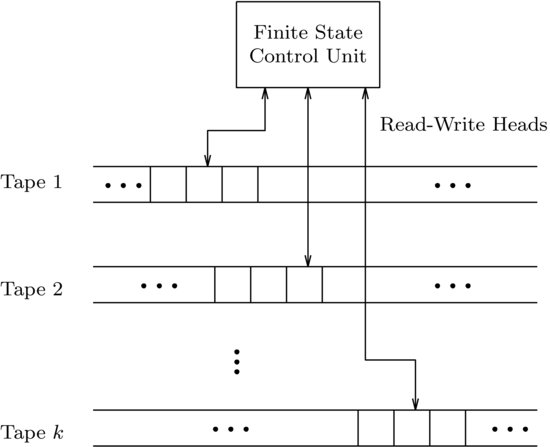
Definition 1.1 A standard multitape Turing machine, M (see Figure 1.2), is an algebraic system defined by

Figure 1.2 k-tape (k 1) Turing machine

(1.12)

where

1. Q is a finite set of internal states;

2. Σ is a finite set of symbols called the input alphabet. We assume that Σ;

3. Γ is a finite set of symbols called the tape alphabet;

4. δ is the transition function, which is defined by

i if M is a deterministic Turing machine (DTM), then

(1.13)

ii if M is a nondeterministic Turing machine (NDTM), then

(1.14)

where L and R specify the movement of the read-write head left or right. When k=1, it is just a standard one-tape Turing machine;

5. is a special symbol called the blank;

6. is the initial state;

7. is the set of final states.

Thus, Turing machines provide us with the simplest possible abstract model of computation for modern digital (even quantum) computers.

Any effectively computable function can be computed by a Turing machine, and there is no effective procedure that a Turing machine cannot perform. This leads naturally to the following famous Church–Turing thesis, named after Alonzo Church (1903–1995) and Alan Turing (1912–1954):

The Church–Turing thesis: Any effectively computable function can be computed by a Turing machine.

The Church–Turing thesis thus provides us with a powerful tool to distinguish what is computation and what is not computation, what function is computable and what function is not computable, and more generally, what computers can do and what computers cannot do. From a computer science and particularly a cryptographic point of view, we are not just interested in what computers can do, but in what computers can do efficiently. That is, in cryptography we are more interested in practical computable rather than just theoretical computable; this leads to the Cook–Karp thesis.

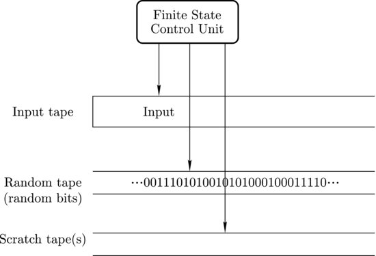
Definition 1.2 A probabilistic Turing machine is a type of nondeterministic Turing machine with distinct states called coin-tossing states. For each coin-tossing state, the finite control unit specifies two possible legal next states. The computation of a probabilistic Turing machine is deterministic except that in coin-tossing states the machine tosses an unbiased coin to decide between the two possible legal next states.

A probabilistic Turing machine can be viewed as a randomized Turing machine, as described in Figure 1.3. The first tape, holding input, is just the same as conventional multitape Turing machine. The second tape is referred to as random tape, containing randomly and independently chosen bits, with probability 1/2 of a 0 and the same probability 1/2 of a 1. The third and subsequent tapes are used, if needed, as scratch tapes by the Turing machine.

Figure 1.3 Probabilistic k-tape (k 1) Turing machine

Definition 1.3 is the class of problems solvable in polynomial-time by a deterministic Turing machine (DTM). Problems in this class are classified to be tractable (feasible) and easy to solve on a computer. For example, additions of any two integers, no matter how big they are, can be performed in polynomial-time, and hence are is in .

Definition 1.4 is the class of problems solvable in polynomial-time on a nondeterministic Turing machine (NDTM). Problems in this class are classified to be intractable (infeasible) and hard to solve on a computer. For example, the Traveling Salesman Problem (TSP) is in , and hence it is hard to solve.

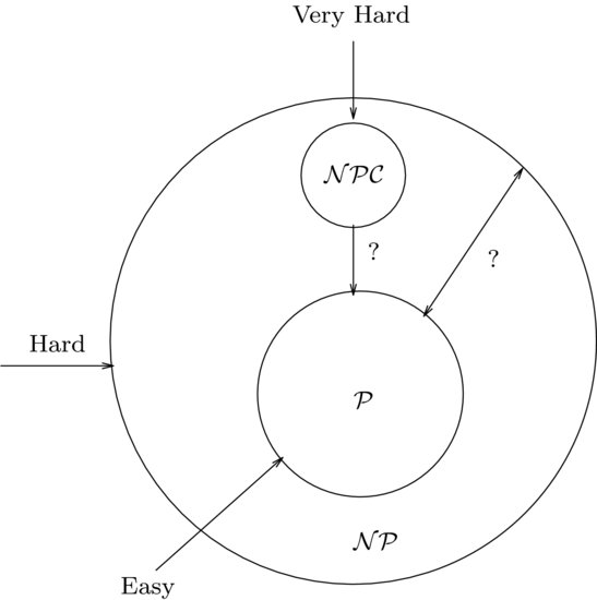
In terms of formal languages, we may also say that is the class of languages where the membership in the class can be decided in polynomial-time, whereas is the class of languages where the membership in the class can be verified in polynomial-time. It seems that the power of polynomial-time verifiable is greater than that of polynomial-time decidable, but no proof has been given to support this statement (see Figure 1.4). The question of whether or not is one of the greatest unsolved problems in computer science and mathematics, and in fact it is one of the seven Millennium Prize Problems proposed by the Clay Mathematics Institute in Boston in 2000, each with one-million US dollars.

Figure 1.4 The Versus problem

Definition 1.5 is the class of problems solvable by a deterministic Turing machine (DTM) in time bounded by .

Definition 1.6 A function f is polynomial-time computable if for any input w, f(w) will halt on a Turing machine in polynomial-time. A language A is polynomial-time reducible to a langauge B, denoted by A B, if there exists a polynomial-time computable function such that for every input w,

The function f is called the polynomial-time reduction of A to B.

Definition 1.7 A language/problem L is -complete, denoted by , if it satisfies the following two conditions:

1. ,

2. .

Definition 1.8 A problem D is -hard, denoted by , if it satisfies the following condition:

where d may be in , or may not be in . Thus, -hard means at least as hard as any -problem, although it might, in fact, be harder.

Definition 1.9 is the class of problems solvable in expected polynomial-time with one-sided error by a probabilistic (randomized) Turing machine (PTM). By “one-sided error” we mean that the machine will answer “yes” when the answer is “yes” with a probability of error <1/2, and will answer “no” when the answer is “no” with zero probability of error.

Definition 1.10 is the class of problems solvable in expected polynomial-time with zero error on a probabilistic Turing machine (PTM). It is defined by = co-, where co- is the complement of . By “zero error” we mean that the machine will answer “yes” when the answer is “yes” (with zero probability of error), and will answer “no” when the answer is “no” (also with zero probability of error). But note that the machine may also answer “?”, which means that the machine does not know if the answer is “yes” or “no.” However, it is guaranteed that in at most half of simulation cases the machine will answer “?.” is usually referred to as an elite class, because it also equals to the class of problems that can be solved by randomized algorithms that always give the correct answer and run in expected polynomial-time.

Definition 1.11 is the class of problems solvable in expected polynomial-time with two-sided error on a probabilistic Turing machine (PTM), in which the answer always has probability at least , for some fixed δ > 0 of being correct. The “” in stands for “bounded away the error probability from ”; for example, the error probability could be .

It is widely believed, although no proof has been given, that problems in are computationally tractable, whereas problems not in (beyond) are computationally intractable. This is the famous Cook–Karp thesis, named after Stephen Cook and Richard Karp:

The Cook–Karp thesis. Any computationally tractable problem can be computed by a Turing machine in deterministic polynomial-time.

Thus, problems in are tractable whereas problems in are intractable. However, there is not a clear cut line between the two types of problems. This is exactly the versus problem, mentioned earlier.

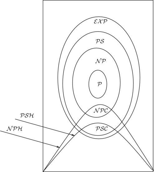
Similarly, one can define the classes of problems of -Space, -Space, -Space Complete, and -Space Hard. We shall use to denote the set of -Complete problems, the set of -Space Complete problems, the set of -Hard problems, and the set of -Space Hard problems. The relationships among the classes , , , , , , and may be described as in Figure 1.5.

Figure 1.5 Conjectured relationships among classes , and , etc.

It is clear that a time class is included in the corresponding space class since one unit is needed for the space by one square. Although it is not known whether or not , it is known that . It is generally believed that

(1.15)

Besides the proper inclusion , it is not known whether any of the other inclusions in the above hierarchy is proper. Note that the relationship of and is not known, although it is believed that .

Problems for Section 1.2

1. Explain why the Church–Turing thesis cannot be proved to be true.

2. Explain why, if any one of the problems in can be solved in , then all the problems in can be solved in .

3. Show that .

4. Prove or disprove .

5. In number theoretic computation, it is reasonable to measure how many bit operations a number theoretic algorithm requires, rather than just how many arithmetic operation it requires. Let A and B both have β (or at least one of them has β) bits. Show that the bit operations for the multiplication of two β numbers can be as follows:

1. if an ordinary method is used;

2. if a simple divide-and-conquer method is used;

3. if a fast method (e.g., Fourier transforms) is used.

6. Show that the addition, subtraction, and division of two integers can be done in polynomial-time.

7. Show that the polynomial factorization (not integer factorization) can be done in polynomial-time.

8. Show that matrix multiplications can be done in polynomial-time.

1.3 What is Computational Number Theory?

Computational number theory is a new branch of mathematics. Informally, it can be regarded as a combined and disciplinary subject of number theory and computer science, particularly computation theory, including the theory of classical electronic computing, quantum computing, and biological computing:

Computational Number Theory := Number Theory Computation Theory
Primality Testing	Elementary Number Theory	Computability Theory
Integer Factorization	Algebraic Number Theory	Complexity Theory
Discrete Logarithms	Combinatorial Number Theory	Infeasibility Theory
Elliptic Curves	Analytic Number Theory	Computer Algorithms
Conjecture Verification	Arithmetic Algebraic Geometry	Computer Architectures
Theorem Proving	Probabilistic Number Theory	Quantum Computing
	Applied Number Theory	Biological Computing

Basically, any topic in number theory where computation plays a central role can be regarded as a topic in computational number theory. Computational number theory aims at either using computing techniques to solve number-theoretic problems, or using number-theoretic techniques to solve computer science problems. We concentrate in this book on using computing techniques to solve number-theoretic problems that have connections and applications in modern public-key cryptography. Typical questions or problems in this category of computational number theory include:

1. Primality Testing Problem (PTP). PTP can be formally defined as follows:

(1.16)

Theoretically speaking, PTP can be solved in polynomial-time, that is, PTP can be solved efficiently on a computer. However, it may still be difficult to decide whether or not a large number is prime. Call a number a Mersenne prime if it is of the form

(1.17)

where p is prime and 2p−1 is also prime. To date, only 47 such p have been found (see Table 1.4); the first 4 were found 2500 years ago. Note that 243112609−1 is not only the largest known Mersenne prime, but also the largest known prime in the world to date. The search for the largest Mersenne prime and/or the largest prime has always been a hot topic in computational number theory. EFF (Electronic Frontier Foundation) has offered in total 550 000 US dollars to the first individual or organization who can find the following large primes:

Prizes	Conditions for the New Primes
$50000	at least 1000000 digits
$100000	at least 10000000 digits
$150000	at least 100000000 digits
$250000	at least 1000000000 digits

The first prize was claimed by Nayan Hajratwala in Michigan in 1996, who found the 38th Mersenne prime 26972593−1 with 2098960 digits, the second prize was claimed by Edson Smith at UCLA in 2008, who found the 46th Mersenne prime 242643801−1 with 12837064 digits. The remaining two prizes remain unclaimed. Of course, we still do not know if there are infinitely many Mersenne primes.

2. Integer Factorization Problem (IFP). IFP can be formally defined as follows:

(1.18)

The IFP assumption is that given the positive integer n>1, it is hard to find its nontrivial factor(s), that is,

Note that in IFP, we aim at finding just one nontrivial factor A (not necessarily a prime factor) of n. The Fundamental Theorem of Arithmetic asserts that any positive integer n>1 can be uniquely written into the following standard prime factorization form:

(1.19)

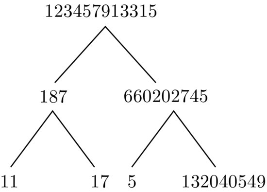
where p1<p2<...<pk are primes, and are positive integers. Clearly, recursively performing the operations of primality testing and integer factorization, n can be eventually written in its standard prime factorization form, say, if we wish to factor 123457913315, the recursive process can be shown in Figure 1.6. So, if we define the Prime Factorization Problem (PFP) as follows:

(1.20)

then

Although PTP can be solved efficiently in polynomial-time, IFP cannot be solved in polynomial-time. Finding polynomial-time factoring algorithms is one of the most important research topics in computational number theory. At present, no polynomial-time algorithm for factoring has been found and no one has yet proved that such an algorithm exists. The current world record for integer factorization is the RSA-768 (a number with 768 bits and 232 digits):

123018668453011775513049495838496272077285356959533479219732245

215172640050726365751874520219978646938995647494277406384592519

255732630345373154826850791702612214291346167042921431160222124

0479274737794080665351419597459856902143413

=

33478071698956898786044169848212690817704794983713768568912431

388982883793878002287614711652531743087737814467999489

3674604366679959042824463379962795263227 9158164343087642676032

283815739666511279 233373417143396810270092798736308917.

It was factored on 9 Dec 2009. The factoring process requires about 1020 operations and would need about 2000 years of computation on a single core 2.2 GHz AMD Opteron.

3. Discrete Logarithm Problem (DLP). According to historical records, logarithms over the set of real numbers were first invented in the 16th century by the Scottish mathematician John Napier (1550–1617). We define k to be the logarithm to the base x of y

(1.21)

if and only if

(1.22)

So the Logarithm Problem (LP) over may be defined as follows:

(1.23)

For example, log319683=9, since 39=19683. LP over is easy to solve, since

(1.24)

where the natural logarithms can be calculated efficiently by the following formula (of course, depending on their accuracy):

(1.25)

For example,

We can always get a result at certain level of accuracy. The Discrete Logarithm Problem over the multiplicative group , discussed in this book, is completely different from the traditional one we just discussed. Let

(1.26)

DLP may be defined as follows:

(1.27)

The DLP assumption is that

The following are some small and simple examples of DLP:

As can be seen, in the first example, the required discrete logarithm does not exist, whereas in the last example, the required discrete logarithms are not unique. In what follows, we give a somewhat larger example of DLP: Let

p= (739. 7149- 736)/3,

7a 127402180119973946824269244334322849749382042586931621654

      557735290322914679095998681860978813046595166455458144280

      588076766033781 (mod p),

7b 180162285287453102444782834836799895015967046695346697313

      025121734059953772058475958176910625380692101651848662362

      1379340 26803049 (mod p).

Find 7ab. To compute 7ab, we need either to find a from 7a mod p or b from 7b mod p, so that we can calculate 7ab=(7a)b=(7b)a. This problem was proposed by McCurley in 1990 and solved by Weber in 1998. The answer to 7ab is:

7ab=381272804111900141380783915079296341939986435510186702850

      563756150455239669294039221021725140532709288726394263700

      63532797740808.

It is obtained by first finding

a=618586908596518832735933316520379042679876430695217134591

  462221849525998156144877820757492182909777408338791850457

  946749734 (mod p-1).

4. Elliptic Curve Discrete Logarithm Problem (ECDLP). Elliptic Curve Discrete Logarithm Problem (ECDLP) is a very natural generalization of the Discrete Logarithm Problem (DLP) from multiplication group to the elliptic curve groups E(), E(), or E(). Let E be an elliptic curve

(1.28)

over a field , denoted by E\. A straight line (nonvertical) L connecting points p and Q intersects the elliptic curve E at a third point R, and the point P Q is the reflection of R in the x-axis. That is, if R=(x3, y3), then P Q = (x3, -y3) is the reflection of R in the x-axis. Note that a vertical line, such as L' or L'', meets the curve at two points (not necessarily distinct), and also at the point at infinity E (we may think of the point at infinity as lying far off in the direction of the y-axis). The line at infinity meets the curve at the point E three times. Of course, the nonvertical line meets the curve at three points in the XY plane. Thus, every line meets the curve at three points. The algebraic formula for computing P3(x3, y3)=P1(x1, y1)+P2(x2, y2) on E is as follows:

(1.29)

where

(1.30)

Given E and P E, it is easy to find Q=kP, which is of course also in E. For example, to compute Q=105P, we first let

and then perform the operations as follows:

1: Q P + 2Q Q P	Q = P
1: Q P+2Q c P+2P	Q = 3P
0: Q 2Q Q 2(P+2P)	Q = 6P
1: Q P+2Q Q P+2(2(P+2P))	Q = 13P
0: Q 2Q Q 2(P+2(2(P+2P)))	Q = 26P
0: Q 2Q Q 2(2(P+2(2(P+2P))))	Q = 52P
1: Q P+2Q Q P+2(2(2(P+2(2(P+2P)))))	Q = 105P.

This gives the required result Q=P+2(2(2(P+2(2(P+2P)))))=105P. As can be seen, given (E\ , k, P) it is easy to compute

(1.31)

However, it is hard to find k given (E\ , P, Q). This is the Elliptic Curve Discrete Logarithm Problem (ECDLP), which may be formally defined as follows (let E be an elliptic curve over finite field ):

(1.32)

The ECDLP assumption asserts that

Suppose that we are given

with

then it is easy to find

since the finite field is small. However, when the finite field is large, such as

on E\ , where

p=1550031797834347859248576414813139942411,

a=1399267573763578815877905235971153316710,

b=1009296542191532464076260367525816293976,

xP=1317953763239595888465524145589872695690,

yP=434829348619031278460656303481105428081,

xQ=1247392211317907151303247721489640699240,

yQ=207534858442090452193999571026315995117.

In this case, it is very hard to find k. Certicom Canada offered 20000 US dollars to the first individual or organization to find the correct value of k. More Certicom prize problems, along with this line, may be found in Table 1.5 (the above-mentioned $20000 prize curve corresponds to ECCp-131, as p has 131-bits in this example):

5. The Root Finding Problem (RFP). The k-th Root Finding Problem (RFP), or RFP for short, may be defined as follows:

(1.33)

If the prime factorization of N is known, one can compute the Euler function (N) and solve the linear Diophantine equation ku- (N)v=1 in u and v, and the computation x yu (mod N) gives the required value. Thus, if IFP can be solved in polynomial-time, then RFP can also be solved in polynomial-time:

The security of RSA relies on the intractability of IFP, and also on RFP; if any one of the problems can be solved in polynomial-time, RSA can be broken in polynomial-time.

6. The Square Root Problem (SQRT) Let y QRN, where QRN denotes the set of quadratic residues modulo n, which should be introduced later. The SQRT Problem is to find an x such that

(1.34)

That is,

(1.35)

When n is prime, the SQRT Problem can be solved in polynomial-time. However, when n is composite one needs to factor n first. Thus, if IFP can be solved in polynomial-time, SQRT can also be solved in polynomial-time:

On the other hand, if SQRT can be solved in polynomial-time, IFP can also be solved in polynomial-time:

That is,

It is precisely this intractability of SQRT Problem that Rabin used to construct his cryptosystem in 1979.

7. Modular Polynomial Root Finding Problem (MPRFP). It is easy to compute the integer roots of a polynomial in one variable over :

(1.36)

but the following Modular Polynomial Root Finding Problem (MPRFP), or the MPRFP for short, can be hard:

(1.37)

which aims at finding integer roots (solutions) of the modular polynomial in one variable. This problem can, of course, be extended to find integer roots (solutions) of the modular polynomial in several variables as follows:

(1.38)

Coppersmith, in 1997, developed a powerful method to find all small solutions x0 of the modular polynomial equations in one or two variables of degree δ using the lattice reduction algorithm LLL (we shall discuss Coppersmith’s method later). Of course, for LLL to be run in a reasonable amount of time for finding such x0’s, the values of δ cannot be large.

8. The Quadratic Residuosity Problem (QRP). Let N >1+, gcd (y,N)=1. Then y is a quadratic residue modulo n, denoted by y QRN}, if the quadratic congruence

(1.39)

has a solution in x. If the congruence has no solution in x, then y is a quadratic nonresidue modulo n, denoted by y N. The Quadratic Residuosity Problem (QRP), or QRP for short, is to decide whether or not y QRN:

(1.40)

If n is prime, or the prime factorization of n is known, then QRP can be solved simply by evaluating the Legendre symbol L(y, N). If n is not a prime then one evaluates the Jacobi symbol J(y, N) which, unfortunately, does not reveal if y QRN, that is, J(y, N)=1 does not imply y QRN (it does if n is prime). For example, L(15, 17)=1, so x2 15 (mod 17) is soluble, with x= 21 being the two solutions. However, although J(17, 21)=1 there is no solution for x2 17 (mod 21). Thus, when n is composite, the only way to decide whether or not y QRN is to factor n. Thus, if IFP can be solved in polynomial-time, QRP can also be solved in polynomial-time:

The security of the Goldwasser–Micali probabilistic encryption scheme is based on the intractability of QRP.

9. Shortest Vector Problem (SVP). Problems related to lattices are also often hard to solve. Let denote the space of n-dimensional real vectors a={ a1,a2, ... , an} with usual dot product a . b and Euclidean Norm or length ||a||=(a . a)1/2. n is the set of vectors in with integer coordinates. If A={ a1,a2, ... , an} is a set of linear independent vectors in , then the set of vectors

(1.41)

is a lattice in , denoted by L(A) or L(a1, a2, ..., an). A is called a basis of the lattice. A set of vectors in is a n-dimensional lattice if there is a basis v of n linear independent vectors such that L=L(V). If A={ a1,a2, ... , an} is a set of vectors in a lattice L, then the length of the set A is defined by max(||ai||). A fundamental theorem, due to Minkowski, is as follows.

Theorem 1.1 (Minkowski) There is a universal constant γ, such that for any lattice L of dimension n, v L, v 0, such that

(1.42)

The determinant det(L) of a lattice is the volume of the n-dimensional fundamental parallelepiped, and the absolute constant γ is known as Hermite’s constant.

A natural problem concerned with lattices is the Shortest Vector Problem (SVP), or the SVP for short:

Find the shortest nonzero vector in a high dimensional lattice.

Minkowski’s theorem is just an existence-type theorem and offers no clue on how to find a short or the shortest nonzero vector in a high dimensional lattice. There is no efficient algorithm for finding the shortest nonzero vector, or finding an approximate short nonzero vector. The lattice reduction algorithm LLL can be used to find short vectors, but it is not effective in finding short vectors when the dimension n is large, say, for example, n 100. This allows lattices to be used in the design of cryptographic systems and in fact, several cryptographic systems, such as NTRU and the Ajtai–Dwork system, are based on the intractability of finding the shortest nonzero vector in a high dimensional lattice.

Table 1.5 Some Certicom ECDLP challenge problems

Figure 1.6 Prime factorization of 123457913315

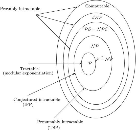
In this book, we are more interested in those number-theoretic problems that are computationally intractable, since the security of modern public-key cryptography relies on the intractability of these problems. A problem is computationally intractable if it cannot be solved in polynomial-time. Thus, from a computational complexity point of view, any problem beyond is intractable. There are, however, different types of intractable problems (see Figure 1.7).

1. Provable intractable problems: Problems that are Turing computable but can be shown in (-pace), (-pace), (exponential time) and so on, of course outside , are provably and certainly intractable. Note that although we do not know if = , we know = .

2. Presumably intractable problems: Problems in but outside of , particularly those problems in (-complete) such as the Traveling Salesman Problem, the Knapsack Problem, and the Satisfiability Problem, are presumably intractable, since we do not know whether or not = . If = , then all problems in will no longer be intractable. However, it is more likely that . From a cryptographic point of view, it would be nice if encryption schemes could be designed to be based on some -complete problems, since these types of schemes can be difficult to break. Experience, however, tells us that very few encryption schemes are based on -complete problems.

3. Conjectured intractable problems: By conjectured intractable problems we mean that the problems are currently in -complete, but no-one can prove they must be in -complete; they may be in if efficient algorithms are invented for solving these problems. Typical problems in this category include the Integer Factorization Problem (IFP), the Discrete Logarithm Problem (DLP), and the Elliptic Curve Discrete Logarithm Problem (ECDLP). Again, from a cryptographic point of view, we are more interested in this type of intractable problem and, in fact, the IFP, DLP, and ECDLP are essentially the only three intractable problems that are practical and widely used in commercial cryptography. For example, the most famous and widely used RSA cryptographic system relies for its security on the intractability of the IFP problem.

Figure 1.7 Tractable and intractable problems

The difference between the presumably intractable problems and the conjectured intractable problems is important and should not be confused. For example, both TSP and IFP are intractable, but the difference between TSP and IFP is that TSP has been proved to be -complete whereas IFP is only conjectured to be -complete. IFP may be -complete, but also may not be -complete.

Finally, we present a complexity measure of number-theoretic problems in big- notation.

Definition 1.12 Let

(1.43)

Define

(1.44)

if there exists c >0 with

(1.45)

Definition 1.13 Let

(1.46)

where α [0,1], c >0.

1. If a problem can be solved by an algorithm in expected running time

(1.47)

then the algorithm is polynomial-time algorithm(or efficient algorithm), and the corresponding problem is an easy problem (i.e., the problem can be solved easily).

It is also often the case that ((log n)k) is used with k constant to represent polynomial-time complexity. For example, the multiplication of two log n-bit numbers by ordinary method takes time ((log n)2), the fastest known multiplication method has a running time of

2. If a problem can be solved by an algorithm in expected running time

(1.48)

then the algorithm is an exponential-time algorithm(or an inefficient algorithm), and the corresponding problem is a hard problem (i.e., the problem is hard to solve).

Note that since log n is the length of input, ((log n)12) is polynomial-time complexity, whereas ((n)0.1) is not, since ((n)^{0.1}) = (20.1 log n}), an exponential complexity.

3. An algorithm is of subexponential-time complexity if

(1.49)

Subexponential-time complexity is an important and interesting class between the two extremes, and in fact, many of the number theoretic algorithms discussed in this book, such as the algorithms for integer factorization and discrete logarithms, fall into this special class, which is slower than polynomial-time but faster than exponential-time.

Subexponential-time complexity is an important complexity class in computational number theory and, in fact, the best algorithms for IFP and DLP run in subexponential-time. For ECDLP, we even do not have a subexponential-time algorithm.

Problems for Section 1.3

1. Prove or disprove that

1. there are infinitely many Mersenne prime numbers;

2. there are infinitely many Mersenne composite numbers.

Find the 48th Mersenne prime.

2. What is the difference between the Integer Factorization Problem and the Prime Factorization Problem?

3. What is the difference between the Discrete Logarithm Problem and the Elliptic Discrete Logarithm Problem.

4. Show that solving the Square Root Problem is equivalent to that of the Integer Factorization Problem.

5. Show that solving the Quadratic Residuosity Problem is equivalent to that of the Integer Factorization Problem.

6. Find all the prime factors of the following numbers:

1. 11111111111 (the number consisting of eleven 1)

2. 111111111111 (the number consisting of twelve 1)

3. 1111111111111 (the number consisting of thirteen 1)

4. 11111111111111 (the number consisting of fourteen 1)

5. 111111111111111 (the number consisting of fifteen 1)

6. 1111111111111111 (the number consisting of sixteen 1)

7. 11111111111111111 (the number consisting of seventeen 1)

8. Can you find any pattern for the prime factorization of the above numbers?

7. Do you think the Integer Factorization Problem, or more generally the Prime Factorization Problem, are hard to solve? Justify your answer.

8. Can you find some problems that have similar properties or difficulties to the Integer Factorization Problem (we shall explain this in detail in the next section)?

9. Find the discrete logarithm k

such that

and the discrete logarithm k

such that

10. Find the square root y

such that

and the square root y

such that

1.4 What is Modern Cryptography?

Cryptography, one of the main topics of this book, is the art and science of secure data communications over insecure channels. It is a very old subject, as old as our human civilization. The basic scenario of cryptography is that Alice wishes to send a message M to Bob over the insecure public channel, but Eve can eavesdrop on the communications from the public channel:

To stop Eve to reading/understanding the message M (note that no one can stop Even eavesdroping M), Alice first encrypts the plaintext M to ciphertext C, and then sends C to Bob:

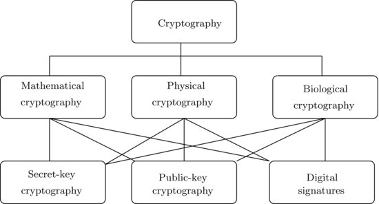
As we just mentioned, cryptography is an old subject, and in fact it has at least 5000 years of history, however, in this book we are more interested in modern cryptography. By modern cryptography, we mean the cryptography studied and invented mainly after the 1970s. Often these types of cryptography are based on advanced and sophisticated mathematics, so we call it mathematical cryptography. More specifically, we call it number-theoretic cryptography if its construction and security are based on the concepts and results in number theory. Of course, modern cryptography may also be based on, say for example, quantum physics and molecular biology, in which case, we may call it quantum cryptography, or biological (DNA) cryptography. Traditionally, cryptography is meant to be secret-key cryptography, in which the encryption and decryption use the same key. By the same key, we mean the encryption key, say, E and the decryption key, say d are polynomial-time computable. That is, given E, d=1/e can be computed easily in polynomial-time. In other words, E and d are polynomial-time equivalent but not physically equivalent. In public-key cryptography, however, E and d are different, as given E, d=1/e cannot be computed in polynomial-time. Of course, they can be computed in exponential-time. So, in public-key cryptography, E and d are not polynomial-time equivalent. Other significant difference between secret-key cryptography and public-key cryptography is that public-key cryptography is normally not only useful for encryption, but is also useful for digital signatures. Figure 1.8 shows the types of cryptography and the relationships among the different types of cryptography.

Figure 1.8 Types of cryptography

Now let us take RSA as an example to illustrate the classification of different type of cryptography. First of all, RSA is a type of mathematical cryptography, more specifically it is a type of number-theoretic cryptography, as its construction and security are all based on the infeasible number-theoretic problem – the Integer Factorization Problem. Secondly, RSA is public-key cryptography and, in fact, it is the first practical, widely used, and still unbreakable public-key cryptography and was invented in 1977 by Rivet, Shamir, and Adleman, then all at MIT. Let M be a plaintext message. To encrypt the M, one computes

(1.50)

where E is the encryption key, and both E and n are public. (The notation a b (mod n) reads “A is congruent to B modulo n.” Congruences will be studied in detail in Section 2.4.) To decrypt the encrypted message C, one computes

(1.51)

where d is the private decryption key satisfying

(1.52)

where (n) is Euler’s -function ( (n), for n 1, is defined to be the number of positive integers not exceeding n which are relatively prime to n; see Definition 2.31). By (1.52), we have ed = 1 + k (n) for some integer k. By Euler’s theorem (see Theorem 2.112), M (n) 1 (mod n), we have Mk (n) 1 (mod n). Thus,

(1.53)

For those who do not have the private key but can factor n, say for example, n=pq, they can find d by computing

(1.54)

and hence, decrypt the message.

Remarkably enough, RSA can also be easily used to obtain digital signatures: Just use the encryption key E and decryption key d in the opposite direction:

1. Signature generation;

(1.55)

where S is the digital signature, which can only be generated by the one who has the private key d.

2. Signature verification;

(1.56)

Anyone can easily verify the signature S, as the verification key is the public key E.

Problems for Section 1.4

1. Why can secret-key cryptography not be used for obtaining digital signatures?

2. Can all the public-key cryptographic schemes be used for obtaining digital signatures?

3. In term of computational complexity, explain why d cannot be computed from E in polynomial-time, given ed 1 (mod (n)) where n=pq with p, q prime numbers.

4. Explain why the security of RSA relies on the infeasibity of the prime factorization of the modulus n.

5. Explain why RSA is only computationally unbreakable, not absolutely unbreakable.

6. Can the RSA encryption exponent E be 2? Justify your answer.

7. Modify RSA to allow e=2.

8. Is RSA is unbreakable? Justify your answer.

9. Although the cryptographic schemes discussed this book are mainly based on the hard number-theoretic probems, there are some other cryptographic schemes whose security is based on some other difficult problems. Write essays on

1. DNA-based cryptography

2. chaos-based cryptography

3. optical cryptography

4. quantum cryptography.

1.5 Bibliographic Notes and Further Reading

In this chapter, we have given a general picture of number theory, computation theory, computational number theory, and modern number-theoretic cryptography, each of them in their own right large, well-established, and important subjects.

For more information on number theory, readers may consult [1-3, 5-12, 14-23]. For more information on computation theory, particularly computability, complexity, and infeasibiity, see e.g., [24-39]. For more information on computational number theory, see for example, [13,14, 23, 27, 38, 40-50]. For more information on cryptography, it is suggested readers consult [51-66].

References

1. T. M. Apostol, Introduction to Analytic Number Theory, Corrected 5th Printing, Undergraduate Texts in Mathematics, Springer, 1998.

2. A. Baker, A Concise Introduction to the Theory of Numbers, Cambridge University Press, 1984.

3. E. Bombieri, The Riemann Hypothesis, In: J. Carlson, A. Jaffe and A. Wiles, Editors, The Millennium Prize Problems, Clay Mathematics Institute and American Mathematical Society, 2006, pp. 107–128.

4. J. Carlson, A. Jaffe and A. Wiles, The Millennium Prize Problems, American Mathematical Society, 2006.

5. J. R. Chen, “On the representation of a larger even integer as the sum of a prime and the product of at most two primes”, Scientia Sinica 16, 1973, pp. 157–176.

6. H. Davenport, The Higher Arithmetic, 7th Edition, Cambridge University Press, 1999.

7. U. Dudley, A Guide to Elementary Number Theory, Mathematical Association of America, 2010.

8. H. M. Edwards, Higher Arithmetic: Al Algorithmic Introduction to Number Theory, American Mathematical Society, 2008.

9. B. Green and T. Tao, “The Primes Contain Arbitrarily Long Arithmetic Progressions”, Annual of Mathematics, 167, 2, 2008, pp. 481–547.

10. G. H. Hardy and E. M. Wright, An Introduction to Theory of Numbers, 6th Edition, Oxford University Press, 2008.

11. D. Husemöller, Elliptic Curves, Graduate Texts in Mathematics 111, Springer, 1987.

12. K. Ireland and M. Rosen, A Classical Introduction to Modern Number Theory, 2nd Edition, Graduate Texts in Mathematics 84, Springer, 1990.

13. D. E. Knuth, The Art of Computer Programming II – Seminumerical Algorithms, 3rd Edition, Addison-Wesley, 1998.

14. N. Koblitz, A Course in Number Theory and Cryptography, 2nd Edition, Graduate Texts in Mathematics 114, Springer, 1994.

15. W. J. LeVeque, Fundamentals of Number Theory, Dover, 1977.

16. I. Niven, H. S. Zuckerman and H. L. Montgomery, An Introduction to the Theory of Numbers, 5th Edition, Wiley, 1991.

17. J. H. Silverman, A Friendly Introduction to Number Theory, 3rd Edition, Prentice-Hall, 2006.

18. J. H. Silverman, The Arithmetic of Elliptic Curves, 2nd Edition, Graduate Texts in Mathematics 106, Springer, 2009.

19. J. H. Silverman and J. Tate, Rational Points on Elliptic Curves, Undergraduate Texts in Mathematics, Springer, 1992.

20. J. Stillwell, Elements of Number Theory, Springer, 2000.

21. L. C. Washinton, Elliptic Curve: Number Theory and Cryptography, 2nd Edition, CRC Press, 2008.

22. A. Wiles, “Modular Elliptic Curves and Fermat’s last Theorem”, Annals of Mathematics, 141, 1994, pp. 443–551.

23. S. Y. Yan, Number Theory for Computing, 2nd Edition, Springer, 2002.

24. S. Arora and B. Barak, Computational Complexity, Cambridge University Press, 2009.

25. S. Cook, The Complexity of Theorem-Proving Procedures, Proceedings of the 3rd Annual ACM Symposium on the Theory of Computing, New York, 1971, pp. 151–158.

26. S. Cook, The P versus NP Problem, In: J. Carlson, A. Jaffe, and A. Wiles, Editors, The Millennium Prize Problems, Clay Mathematics Institute and American Mathematical Society, 2006, pp. 87–104.

27. T. H. Cormen, C. E. Ceiserson, and R. L. Rivest, Introduction to Algorithms, 3rd Edition, MIT Press, 2009.

28. M. R. Garey and D. S. Johnson, Computers and Intractability – A Guide to the Theory of NP-Completeness, W. H. Freeman and Company, 1979.

29. J. Hopcroft, R. Motwani, and J. Ullman, Introduction to Theory of Computation, Jones and Bartlett Publishers, 2008.

30. J. Hopcroft, R. Motwani, and J. Ullman, Introduction to Automata Theory, Languages, and Computation, 3rd Edition, Addison-Wesley, 2007.

31. P. Linz, An Introduction to Formal Languages and Automata, 3rd Edition, Jones and Bartlett Publishers, 2000.

32. R. Karp, “Reducibility among Combinatorial Problems”, Complexity of Computer Computations. Edited by R. E. Miller and J. W. Thatcher, Plenum Press, New York, 1972, pp. 85–103.

33. C. Petzold, The Annotated Turing: A Guide Tour through Alan Turing’s Historical Paper on Computability and the Turing Machine, Wiley, 2008.

34. G. Rozenberg and A. Salomaa, Cornerstones of Undecidability, Prentice-Hall, 1994.

35. R. Sedgewick and K. Wayne, Algorithms, 4th Edition, Cambridge University Press, 2011.

36. M. Sipser, Introduction to the Theory of Computation, 2nd Edition, Thomson, 2006.

37. A. Turing, “On Computable Numbers, with an Application to the Entscheidungsproblem”, Proceedings of the London Mathematical Society, Series 2 42, 1937, pp. 230–265 and 43, 1937, pp. 544–546.

38. H. S. Wilf, Algorithms and Complexity, 2nd Edition, A. K. Peters, 2002.

39. S. Y. Yan, An Introduction to Formal Languages and Machine Computation, World-Scientific, 1998.

40. L. M. Adleman, “Algorithmic Number Theory – The Complexity Contribution”, Proceedings of the 35th Annual IEEE Symposium on Foundations of Computer Science, IEEE Press, 1994, pp. 88–113.

41. E. Bach and J. Shallit, Algorithmic Number Theory I – Efficient Algorithms, MIT Press, 1996.

42. H. Cohen, A Course in Computational Algebraic Number Theory, Graduate Texts in Mathematics 138, Springer, 1993.

43. R. Crandall and C. Pomerance, Prime Numbers – A Computational Perspective, 2nd Edition, Springer, 2005.

44. M. F. Jones, M. Lal, and W. J. Blundon, “Statistics on Certain Large Primes”, Mathematics of Computation, 21, 97, 1967, pp. 103–107.

45. E. Kranakis, Primality and Cryptography, Wiley, 1986.

46. C. Pomerance, “Computational Number Theory”, Princeton Companion to Mathematics. Edited by W. T. Gowers, Princeton University Press, 2008, pp. 348–362.

47. H. Riesel, Prime Numbers and Computer Methods for Factorization, Birkhäuser, Boston, 1990.

48. V. Shoup, A Computational Introduction to Number Theory and Algebra, Cambridge University Press, 2005.

49. R. D. Silverman, “A Perspective on Computational Number Theory”, Notices of the American Mathematical Society, 38, 6, 1991, pp. 562–568.

50. J. von zur Gathen and J. Gerhard, Modern Computer Algebra, 2nd Edition, Cambridge University Press, 2003.

51. M. Ajtai and C. Dwork, “A Pubic-Key Cryptosystem with Worst-Case/Average-Case Equivalence”, Proceedings of Annual ACM Symposium on Theory of Computing, 1997, pp. 284–293.

52. F. L. Bauer, Decrypted Secrets – Methods and Maxims of Cryptology, 3rd Edition, Springer, 2002.

53. J.A. Buchmann, Introduction to Cryptography, Springer, 2004.

54. H. Cohen and G. Frey, Elliptic and Hyperelliptic Curve Cryptography, Chapman & Hall/CRC, 2006.

55. N. Ferguson, B. Schneier and T. Kohno, Cryptography Engineering, Wiley, 2010.

56. S. Goldwasser and S. Micali, “Probabilistic Encryption”, Journal of Computer and System Sciences, 28, 1984, pp. 270–299.

57. J. Hoffstein, N. Howgrave-Graham, J. Pipher, J. H. Silverman and W. Whyte, “NTRUEncrypt and NTRUSign: Efficient Public Key Algorithmd for a Post-Quantum World”, Proceedings of the International Workshop on Post-Quantum Cryptography (PQCrypto 2006), 23–26 May 2006, pp. 71–77.

58. N. Koblitz, Algebraic Aspects of Cryptography, Springer, 1998.

59. A. J. Menezes, P.C. van Oorschot and S. A. Vanstone, Handbook of Applied Cryptography, CRC Press, 1997.

60. Codes: The Guide to Secrecy from Ancient to Modern Times, CRC Press, 2005.

61. J. Pieprzyk, Hardjono and J. Seberry, Fundamentals of Computer Security, Springer, 2003.

62. J. Rothe, Complexity Theory and Cryptology, Springer, 2005.

63. I. Shparlinski, Number Theoretic Methods in Cryptography, Birkhäuser, 1999.

64. I. Shparlinski, Cryptographic Applications of Analytic Number Theory, Birkhäuser, 2003.

65. M. Stamp and R. M. Low, Applied Cryptanaysis, IEEE Press and Wiley, 2007.

66. A. L. Young, Mathematical Ciphers, American Mathematical Society, 2006.