2.4 Congruence Theory

The notion of congruences was first introduced by Gauss, who gave their definition in his celebrated Disquisitiones Arithmeticae in 1801, though the ancient Greeks and Chinese had the idea first.

Definition 2.34 Let a be an integer and n a positive integer greater than 1. We define “” to be the remainder r when a is divided by n, that is

(2.89)

We may also say that “r is equal to a reduced modulo n”.

Remark 2.7 It follows from the above definition that is the integer r such that and , which was known to the ancient Greeks 2000 years ago.

Example 2.37 The following are some examples of a mod n:

Given the well-defined notion of the remainder of one integer when divided by another, it is convenient to provide a special notion to indicate equality of remainders.

Definition 2.35 Let a and b be integers and n a positive integer. We say that “a is congruent to b modulo n”, denoted by

(2.90)

if n is a divisor of a−b, or equivalently, if . Similarly, we write

(2.91)

if a is not congruent (or incongruent) to b modulo n, or equivalently, if . Clearly, for (resp. ), we can write a = kn+b (resp. ) for some integer K. The integer n is called the modulus.

Clearly,

and

So, the above definition of congruences, introduced by Gauss in his Disquisitiones Arithmeticae, does not offer any new idea other than the divisibility relation, since “” and “” (resp. “” and “”) have the same meaning, although each of them has its own advantages. However, Gauss did present a new way (i.e., congruences) of looking at the old things (i.e., divisibility); this is exactly what we are interested in. It is interesting to note that the ancient Chinese mathematician Ch’in Chiu-Shao (1202–1261) had already noted the idea of congruences in his famous book Mathematical Treatise in Nine Chapters in 1247.

Definition 2.36 If , then b is called a residue of a modulo n. If , b is called the least non-negative residue of a modulo n.

Remark 2.8 It is common, particularly in computer programs, to denote the least non-negative residue of a modulo n by . Thus, if and only if , and, of course, if and only if .

Example 2.38 The following are some examples of congruences or incongruences.

	since
	since
	since

The congruence relation has many properties in common with the of equality relation. For example, we know from high-school mathematics that equality is

1. reflexive: a = a, ;

2. symmetric: if a = b, then b = a, ;

3. transitive: if a = b and b = c, then a = c, .

We shall see that congruence modulo n has the same properties:

Theorem 2.41 Let n be a positive integer. Then the congruence modulo n is

1. reflexive: , ;

2. symmetric: if , then , ;

3. transitive: if and , then , .

Proof:

1. For any integer a, we have , hence .

2. For any integers a and b, if , then a = kn+b for some integer K. Hence b = a−kn = (−k)n+a, which implies , since −k is an integer.

3. If and , then a = k1n+b and b = k2n+c. Thus, we can get

which implies , since is an integer.

Theorem 2.41 shows that congruence modulo n is an equivalence relation on the set of integers . But note that the divisibility relation is reflexive, and transitive but not symmetric; in fact if and then a = b, so it is not an equivalence relation. The congruence relation modulo n partitions into n equivalence classes. In number theory, we call these classes congruence classes, or residue classes.

Definition 2.37 If , then a is called a residue of x modulo n. The residue class of a modulo n, denoted by [a]n (or just [a] if no confusion will be caused), is the set of all those integers that are congruent to a modulo n. That is,

(2.92)

Note that writing is the same as writing .

Example 2.39 Let n = 5. Then there are five residue classes, modulo 5, namely the sets:

,

,

,

,

.

The first set contains all those integers congruent to 0 modulo 5, the second set contains all those congruent to 1 modulo 5, ..., and the fifth (i.e., the last) set contains all those congruent to 4 modulo 5. So, for example, the residue class [2]5 can be represented by any one of the elements in the set

Clearly, there are infinitely many elements in the set [2]5.

Example 2.40 In residue classes modulo 2, [0]2 is the set of all even integers, and [1]2 is the set of all odd integers:

Example 2.41 In congruence modulo 5, we have

We also have

So, clearly, [4]5 = [9]5.

Example 2.42 Let n = 7. There are seven residue classes, modulo 7. In each of these seven residue classes, there is exactly one least residue of x modulo 7. So the complete set of all least residues x modulo 7 is .

Definition 2.38 The set of all residue classes modulo n, often denoted by or , is

(2.93)

Remark 2.9 One often sees the definition

(2.94)

which should be read as equivalent to (2.93) with the understanding that 0 represents [0]n, 1 represents [1]n, 2 represents [2]n, and so on; each class is represented by its least non-negative residue, but the underlying residue classes must be kept in mind. For example, a reference to −a as a member of is a reference to [n−a]n, provided , since .

The following theorem gives some elementary properties of residue classes:

Theorem 2.42 Let n be a positive integer. Then we have

1. [a]n = [b]n if and only if ;

2. Two residue classes modulo n are either disjoint or identical;

3. There are exactly n distinct residue classes modulo n, namely, [0]n, [1]n, [2]n, , and they contain all of the integers.

Proof:

1. If , it follows from the transitive property of congruence that an integer is congruent to a modulo n if and only if it is congruent to b modulo n. Thus, [a]n = [b]n. To prove the converse, suppose [a]n = [b]n. Because and , Thus, .

2. Suppose [a]n and [b]n have a common element c. Then and . From the symmetric and transitive properties of congruence, it follows that . From part (1) of this theorem, it follows that [a]n = [b]n. Thus, either [a]n and [b]n are disjoint or identical.

3. If a is an integer, we can divide a by n to get

Thus, and so [a]n = [r]n. This implies that a is in one of the residue classes Because the integers are incongruent modulo n, it follows that there are exactly n residue classes modulo n.

Definition 2.39 Let n be a positive integer. A set of integers is called a complete system of residues modulo n, if the set contains exactly one element from each residue class modulo n.

Example 2.43 Let n = 4. Then is a complete system of residues modulo 4, since , , , and . Of course, it can be easily verified that is another complete system of residues modulo 4. It is clear that the simplest complete system of residues modulo 4 is , the set of all non-negative least residues modulo 4.

Example 2.44 Let n = 7. Then

is a complete system of residues modulo 7, for any . To see this let us first evaluate the powers of 3 modulo 7:

3

hence, the result follows from x = 0. Now the general result follows immediately, since (x+3i)−(x+3j) = 3i−3j.

Theorem 2.43 Let n be a positive integer and s a set of integers. s is a complete system of residues modulo n if and only if s contains n elements and no two elements of s are congruent, modulo n.

Proof: If s is a complete system of residues, then the two conditions are satisfied. To prove the converse, we note that if no two elements of s are congruent, the elements of s are in different residue classes modulo n. Since s has n elements, all the residue classes must be represented among the elements of s. Thus, s is a complete system of residues modulo n.

We now introduce one more type of system of residues, the reduced system of residues modulo n.

Definition 2.40 Let [a]n be a residue class modulo n. We say that [a]n is relatively prime to n if each element in [a]n is relatively prime to n.

Example 2.45 Let n = 10. Then the ten residue classes, modulo 10, are as follows:

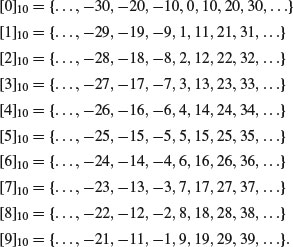
Clearly, [1]10, [3]10, [7]10, and [9]10 are residue classes that are relatively prime to 10.

Proposition 2.1 If a residue class modulo n has one element which is relatively prime to n, then every element in that residue class is relatively prime to n.

Proposition 2.2 If n is prime, then every residue class modulo n (except [0]n) is relatively prime to n.

Definition 2.41 Let n be a positive integer, then is the number of residue classes modulo n, which is relatively prime to n. A set of integers is called a reduced system of residues, if the set contains exactly one element from each residue class modulo n which is relatively prime to n.

Example 2.46 In Example 2.45, we know that [1]10, [3]10, [7]10, and [9]10 are residue classes that are relatively prime to 10, so by choosing −29 from [1]10, −17 from [3]10, 17 from [7]10 and 39 from [9]10, we get a reduced system of residues modulo 10: . Similarly, is another reduced system of residues modulo 10.

One method of obtaining a reduced system of residues is to start with a complete system of residues and delete those elements that are not relatively prime to the modulus n. Thus, the simplest reduced system of residues is just the collections of all integers in the set that are relatively prime to n.

Theorem 2.44 Let n be a positive integer, and s a set of integers. Then s is a reduced system of residues if and only if

1. s contains exactly elements;

2. no two elements of s are congruent ;

3. each element of s is relatively prime to n.

Proof: It is obvious that a reduced system of residues satisfies the three conditions. To prove the converse, we suppose that s is a set of integers having the three properties. Because no two elements of s are congruent, the elements are in different residues modulo n. Since the elements of s are relatively prime n, there are in residue classes that are relatively prime n. Thus, the elements of s are distributed among the residue classes that are relatively prime n, one in each residue class. Therefore, s is a reduced system of residues modulo n.

Corollary 2.3 Let be a reduced system of residues modulo m, and suppose that . Then is also a reduced system of residues modulo n.

Proof: Left as an exercise.

The finite set is closely related to the infinite set . So it is natural to ask if it is possible to define addition and multiplication in and do some reasonable kind of arithmetic there. Surprisingly, the addition, subtraction, and multiplication in will be much the same as that in .

Theorem 2.45 For all and , if and . then

1. ;

2. ;

3. , .

Proof:

1. Write a = kn+b and c = ln+d for some . Then a+c = (k+l)n+b+d. Therefore, a+c = b+d+tn, . Consequently, , which is what we wished to show. The case for subtraction is left as an exercise.

2. Similarly,

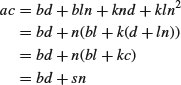
where . Thus, .

3. We prove Part (3) by induction. We have (base step) and (inductive hypothesis). Then by Part (2) we have

Theorem 2.45 is equivalent to the following theorem, since

Theorem 2.46 For all , if [a]n = [b]n, [c]n = [d]n, then

1. ,

2. ,

3. [am]n = [bm]n, .

The fact that the congruence relation modulo n is stable for addition (subtraction) and multiplication means that we can define binary operations, again called addition (subtraction) and multiplication on the set of of equivalence classes modulo n as follows (in case only one n is being discussed, we can simply write [x] for the class [x]n):

(2.95)

(2.96)

(2.97)

Example 2.47 Let n = 12, then

In many cases, we may still prefer to write the above operations as follows:

We summarize the properties of addition and multiplication modulo n in the following two theorems.

Theorem 2.47 The set of integers modulo n has the following properties with respect to addition:

1. Closure: , for all ;

2. Associative: ([x]+[y])+[z] = [x]+([y]+[z]), for all ;

3. Commutative: [x]+[y] = [y]+[x], for all ;

4. Identity, namely, [0];

5. Additive inverse: −[x] = [−x], for all .

Proof: These properties follow directly from the stability and the definition of the operation in .

Theorem 2.48 The set of integers modulo n has the following properties with respect to multiplication:

1. Closure: , for all ;

2. Associative: , for all ;

3. Commutative: , for all ;

4. Identity, namely, [1];

5. Distributivity of multiplication over addition: , for all .

Proof: These properties follow directly from the stability of the operation in and the corresponding properties of .

The division a/b (we assume a/b is in lowest terms and ) in , however, will be more of a problem; sometimes you can divide, sometimes you cannot. For example, let n = 12 again, then

	(no problem),
	(impossible).

Why is division sometimes possible (e.g., ) and sometimes impossible (e.g., )? The problem is with the modulus n; if n is a prime number, then the division is always possible and unique, whilst if n is a composite then the division may be not possible or the result may be not unique. Let us observe two more examples, one with n = 13 and the other with n = 14. First note that if and only if is possible, since multiplication modulo n is always possible. We call the multiplicative inverse (or the modular inverse) of b modulo n. Now let n = 13 be a prime, then the following table gives all the values of the multiplicative inverses for :

This means that division in is always possible and unique. On the other hand, if n = 14 (the n now is a composite), then

This means that only the numbers 1, 3, 5, 9, 11 and 13 have multiplicative inverses modulo 14, or equivalently only those divisions by 1, 3, 5, 9, 11 and 13 modulo 14 are possible. This observation leads to the following important results:

Theorem 2.49 The multiplicative inverse 1/b modulo n exists if and only if .

But how many b’s satisfy ? The following result answers this question.

Corollary 2.4 There are numbers b for which exists.

Example 2.48 Let n = 21. Since , there are twelve values of b for which exists. In fact, the multiplicative inverse modulo 21 only exists for each of the following b:

Corollary 2.5 The division a/b modulo n (assume that a/b is in lowest terms) is possible if and only if exists, that is, if and only if .

Example 2.49 Compute whenever it is possible. By the multiplicative inverses of in the previous table, we just need to calculate :

As can be seen, addition (subtraction) and multiplication are always possible in , with n>1, since is a ring. Note also that with n prime is an Abelian group with respect to addition, and all the nonzero elements in form an Abelian group with respect to multiplication (i.e., a division is always possible for any two nonzero elements in if n is prime); hence with n prime is a field. That is:

Theorem 2.50 is a field if and only if n is prime.

The above results only tell us when the multiplicative inverse 1/a modulo n is possible, without mentioning how to find the inverse. To actually find the multiplicative inverse, we let

(2.98)

which is equivalent to

(2.99)

Since

(2.100)

Thus, finding the multiplicative inverse is the same as finding the solution of the linear Diophantine equation ax−ny = 1, which, as we know, can be solved by using the continued fraction expansion of a/n or by using Euclid’s algorithm.

Example 2.50 Find

1. ,

2. .

Solution

1. Since

we only need to find x and y in

To do so, we first use the Euclid’s algorithm to find as follows:

Since , by Theorem 2.49, the equation 154x−801y = 1 is soluble. We now rewrite the above resulting equations

and work backwards on the above new equations

So, . That is,

2. By Part (1) above, we have

The above procedure used to find the x and y in ax+by = 1 can be generalized to find the x and y in ax+by = c; this procedure is usually called the extended Euclid’s algorithm.

Congruences have much in common with equations. In fact, the linear congruence is equivalent to the linear Diophantine equation ax−ny = b. That is,

(2.101)

Thus, linear congruences can be solved by using the continued fraction method just as for linear Diophantine equations.

Theorem 2.51 Let . If , then the linear congruence

(2.102)

has no solution.

Proof: We will prove the contrapositive of the assertion: If has a solution, then . Suppose that s is a solution. Then , and from the definition of the congruence, , or from the definition of divisibility, as−b = kn for some integer K. Since and , it follows that .

Theorem 2.52 Let . Then the linear congruence has solutions if and only if .

Proof: Follows from Theorem 2.51.

Theorem 2.53 Let . Then the linear congruence has exactly one solution.

Proof: If , then there exist x and y such that ax+ny = 1. Multiplying by b gives

As a(xb)−b is a multiple of n, or , the least residue of xb modulo n is then a solution of the linear congruence. The uniqueness of the solution is left as an exercise.

Theorem 2.54 Let and suppose that . Then the linear congruence

(2.103)

has exactly d solutions modulo n. These are given by

(2.104)

where t is the solution, unique modulo n/d, of the linear congruence

(2.105)

Proof: By Theorem 2.52, the linear congruence has solutions since . Now let t be be such a solution, then t+k(n/d) for are also solutions, since

Example 2.51 Solve the linear congruence . Notice first that

Now we use the Euclid’s algorithm to find as follows:

Since and , by Theorem 2.31, the equation 154x−801y = 22 is soluble. Now we rewrite the above resulting equations

and work backwards on the above new equations

So, . By Theorems 2.53 and 2.54, is the only solution to the simplified congruence:

since . By Theorem 2.54, there are, in total, eleven solutions to the congruence , as follows:

Thus,

are the eleven solutions to the original congruence .

Remark 2.10 To find the solution for the linear Diophantine equation

(2.106)

is equivalent to finding the quotient of the modular division

(2.107)

which is, again, equivalent to finding the multiplicative inverse

(2.108)

because if modulo n exists, the multiplication is always possible.

Theorem 2.55 (Fermat’s little theorem) Let a be a positive integer and . If p is prime, then

(2.109)

Proof: First notice that the residues modulo p of are in some order, because no two of them can be equal. So, if we multiply them together, we get

This means that

Now we can cancel the (p−1)! since , and the result thus follows.

There is a more convenient and more general form of Fermat’s little theorem:

(2.110)

for . The proof is easy: If , we simply multiply (2.109) by a. If not, then . So .

Fermat’s theorem has several important consequences which are very useful in compositeness; one of the these consequences is as follows:

Corollary 2.6 (Converse of the Fermat little theorem, 1640) Let n be an odd positive integer. If and

(2.111)

then n is composite.

Remark 2.11 In 1640, Fermat made a false conjecture that all the numbers of the form were prime. Fermat really should not have made such a “stupid” conjecture, since F5 can be relatively easily verified to be composite, just by using his own recently discovered theorem – Fermat’s little theorem:

Thus, by Fermat’s little theorem, 232+1 is not prime!

Based on Fermat’s little theorem, Euler established a more general result in 1760:

Theorem 2.56 (Euler’s theorem) Let a and n be positive integers with . Then

(2.112)

Proof: Let be a reduced residue system modulo n. Then is also a residue system modulo n. Thus we have

since , being a reduced residue system, must be congruent in some order to . Hence,

which implies that

It can be difficult to find the order1 of an element a modulo n but sometimes it is possible to improve (2.112) by proving that every integer a modulo n must have an order smaller than the number – this order is actually a number that is a factor of .

Theorem 2.57 (Carmichael’s theorem) Let a and n be positive integers with . Then

(2.113)

where is Carmichael’s function, given in Definition 2.32.

Proof: Let . We shall show that

for , since this implies that . If or a power of an odd prime, then by Definition 2.32, , so . Since , . The case that is a power of 2 greater than 4 is left as an exercise.

Note that will never exceed and is often much smaller than ; it is the value of the largest order it is possible to have.

Example 2.52 Let a = 11 and n = 24. Then , . So,

That is, ord24(11) = 2.

In 1770 Edward Waring (1734–1793) published the following result, which is attributed to John Wilson (1741–1793).

Theorem 2.58 (Wilson’s theorem) If p is a prime, then

(2.114)

Proof: It suffices to assume that p is odd. Now to every integer a with 0<a<p there is a unique integer with such that . Further if then whence a = 1 or a = p−1. Thus the set can be divided into (p−3)/2 pairs with . Hence we have , and so , as required.

Theorem 2.59 (Converse of Wilson’s theorem) If n is an odd positive integer greater than 1 and

(2.115)

then n is a prime.

Remark 2.12 Prime p is called a Wilson prime if

(2.116)

where

is an integer, or equivalently if

(2.117)

For example, p = 5, 13, 563 are Wilson primes, but 599 is not since

It is not known whether there are infinitely many Wilson primes; to date, the only known Wilson primes for are p = 5, 13, 563. A prime p is called a Wieferich prime, named after A. Wieferich, if

(2.118)

To date, the only known Wieferich primes for are p = 1093 and 3511.

In what follows, we shall show how to use Euler’s theorem to calculate the multiplicative inverse modulo n, and hence the solutions of a linear congruence.

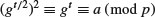
Theorem 2.60 Let x be the multiplicative inverse 1/a modulo n. If , then

(2.119)

is given by

(2.120)

Proof: By Euler’s theorem, we have . Hence

and is the multiplicative inverse of a modulo n, as desired.

Corollary 2.7 Let x be the division b/a modulo n (b/a is assumed to be in lowest terms). If , then

(2.121)

is given by

(2.122)

Corollary 2.8 If , then the solution of the linear congruence

(2.123)

is given by

(2.124)

Example 2.53 Solve the congruence . First note that because , the congruence has exactly one solution. Using (2.124) we get

Example 2.54 Solve the congruence . First note that as and , the congruence has exactly five solutions modulo 135. To find these five solutions, we divide by 5 and get a new congruence

To solve this new congruence, we get

Therefore, the five solutions are as follows:

Next we shall introduce a method for solving systems of linear congruences. The method, widely known as the Chinese Remainder theorem (or just CRT, for short), was discovered by the ancient Chinese mathematician Sun Tsu (who lived sometime between 200 B.C. and 200 A.D.).

Theorem 2.61 (The Chinese Remainder theorem CRT) If m1, m2, ..., mn are pairwise relatively prime and greater than 1, and a1, a2, ..., an are any integers, then there is a solution x to the following simultaneous congruences:

(2.125)

If x and are two solutions, then , where M = m1m2...mn.

Proof: Existence: Let us first solve a special case of the simultaneous congruences (2.125), where i is some fixed subscript,

Let ki = m1m2...mi−1mi+1...mn. Then ki and mi are relatively prime, so we can find integers r and s such that rki+smi = 1. This gives the congruences:

Since all divide ki, it follows that xi = rki satisfies the simultaneous congruences:

For each subscript i, , we find such an xi. Now to solve the system of the simultaneous congruences (2.125), set x = a1x1+a2x2+...+anxn. Then for each i, , such that x is a solution of the simultaneous congruences.

Uniqueness: Let be another solution to the simultaneous congruences (2.125), but different from the solution x, so that for each xi. Then for each i. So mi divides for each i; hence the least common multiple of all the mj’s divides . But since the mi are pairwise relatively prime, this least common multiple is the product m. So .

Remark 2.13 If the system of the linear congruences (2.125) is soluble, then its solution can be conveniently described as follows:

(2.126)

where

for .

Example 2.55 Consider the Sun Zi problem:

By (2.126), we have

Hence,

The congruences we have studied so far are a special type of congruence; they are all linear congruences. In this section, we shall study the higher degree congruences, particularly the quadratic congruences.

Definition 2.42 Let m be a positive integer, and let

be any polynomial with integer coefficients. Then a high-order congruence or a polynomial congruence is a congruence of the form

(2.127)

A polynomial congruence is also called a polynomial congruential equation.

Let us consider the polynomial congruence

This congruence holds when x = 2, since

Just as for algebraic equations, we say that x = 2 is a root or a solution of the congruence. In fact, any value of x which satisfies the following condition

is also a solution of the congruence. In general, as in linear congruence, when a solution x0 has been found, all values x for which

are also solutions. But by convention, we still consider them as a single solution. Thus, our problem is to find all incongruent (different) solutions of . In general, this problem is very difficult, and many techniques of solution depend partially on trial-and-error methods. For example, to find all solutions of the congruence , we could certainly try all values (or the numbers in the complete residue system modulo n), and determine which of them satisfy the congruence; this would give us the total number of incongruent solutions modulo n.

Theorem 2.62 Let M = m1m2...mn, where are pairwise relatively prime. Then the integer x0 is a solution of

(2.128)

if and only if x0 is a solution of the system of polynomial congruences:

(2.129)

If x and are two solutions, then , where M = m1m2...mn.

Proof: If , then obviously , for . Conversely, suppose a is a solution of the system

Then f(a) is a solution of the system

and it follows from the Chinese Remainder theorem that . Thus, a is a solution of .

We now restrict ourselves to quadratic congruences, the simplest possible nonlinear polynomial congruences.

Definition 2.43 A quadratic congruence is a congruence of the form:

(2.130)

where . To solve the congruence is to find an integral solution for x which satisfies the congruence.

In most cases, it is sufficient to study the above congruence rather than the following more general quadratic congruence

(2.131)

since if and b is even or n is odd, then the congruence 2.31 can be reduced to a congruence of type (2.130). The problem can even be further reduced to solving a congruence of the type (if , where are distinct primes, and are positive integers):

(2.132)

because solving the congruence(2.132) is equivalent to solving the following system of congruences:

(2.133)

In what follows, we shall be only interested in quadratic congruences of the form

(2.134)

where p is an odd prime and .

Definition 2.44 Let a be any integer and n a natural number, and suppose that . Then a is called a quadratic residue modulo n if the congruence

is soluble. Otherwise, it is called a quadratic non-residue modulo n.

Remark 2.14 Similarly, we can define the cubic residues, and fourth-power residues, etc. For example, a is a Kth power residue modulo n if the congruence

(2.135)

is soluble. Otherwise, it is a Kth power non-residue modulo n.

Theorem 2.63 Let p be an odd prime and a an integer not divisible by p. Then the congruence

(2.136)

has either no solution or exactly two congruence solutions modulo p.

Proof: If x and y are solutions to , then , that is, . Since x2−y2 = (x+y)(x−y), we must have or , that is, . Hence, any two distinct solutions modulo p differ only by a factor of −1.

Example 2.56 Find the quadratic residues and quadratic nonresidues for moduli 5, 7, 11, 15, 23, respectively.

1. Modulo 5, the integers 1, 4 are quadratic residues, whilst 2, 3 are quadratic nonresidues, since

2. Modulo 7, the integers 1, 2, 4 are quadratic residues, whilst 3, 5, 6 are quadratic nonresidues, since

3. Modulo 11, the integers 1, 3, 4, 5, 9 are quadratic residues, whilst 2, 6, 7, 8, 10 are quadratic nonresidues, since

4. Modulo 15, only the integers 1 and 4 are quadratic residues, whilst 2, 3, 5, 6, 7, 8, 9, 10, 11, 12, 13, 14 are all quadratic nonresidues, since

5. Modulo 23, the integers 1, 2, 3, 4, 6, 8, 9, 12, 13, 16, 18 are quadratic residues, whilst 5, 7, 10, 11, 14, 15, 17, 19, 20, 21, 22 are quadratic nonresidues, since

The above example illustrates the following two theorems:

Theorem 2.64 Let p be an odd prime and N(p) the number of consecutive pairs of quadratic residues modulo p in the interval [1, p−1]. Then

(2.137)

Proof: (Sketch) The complete proof of this theorem can be found in [1] and [2]; here we only give a sketch of the proof. Let (RR), (RN), (NR) and (NN) denote the number of pairs of two quadratic residues, of a quadratic residue followed by a quadratic non-residue, of a quadratic non-residue followed by a quadratic residue, of two quadratic non-residues, among pairs of consecutive positive integers less than p, respectively. Then

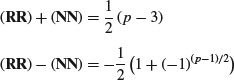
Hence

Remark 2.15 Similarly, let denote the number of consecutive triples of quadratic residues in the interval [1, p−1], where p is odd prime. Then

(2.138)

where .

Example 2.57 For p = 23, there are five consecutive pairs of quadratic residues, namely, (1, 2), (2, 3), (3, 4), (8, 9), and (12, 13), modulo 23; there is also one consecutive triple of quadratic residues, namely, (1, 2, 3), modulo 23.

Theorem 2.65 Let p be an odd prime. Then there are exactly (p−1)/2 quadratic residues and exactly (p−1)/2 quadratic nonresidues modulo p.

Proof: Consider the p−1 congruences:

Since each of the above congruences has either no solution or exactly two congruence solutions modulo p, there must be exactly (p−1)/2 quadratic residues modulo p among the integers . The remaining

positive integers less than p−1 are quadratic nonresidues modulo p.

Example 2.58 Again for p = 23, there are eleven quadratic residues, and eleven quadratic nonresidues modulo 23.

Euler devised a simple criterion for deciding whether an integer a is a quadratic residue modulo a prime number p.

Theorem 2.66 (Euler’s criterion) Let p be an odd prime and . Then a is a quadratic residue modulo p if and only if

Proof: Using Fermat’s little theorem, we find that

and thus . If a is a quadratic residue modulo p, then there exists an integer x0 such that . By Fermat’s little theorem, we have

To prove the converse, we assume that . If G is a primitive root modulo p (G is a primitive root modulo p if ; we shall formally define primitive roots in Section 2.5), then there exists a positive integer t such that . Then

which implies that

Thus, t is even, and so

which implies that a is a quadratic residue modulo p.

Euler’s criterion is not very useful as a practical test for deciding whether or not an integer is a quadratic residue, unless the modulus is small. Euler’s studies on quadratic residues were further developed by Legendre, who introduced the Legendre symbol.

Definition 2.45 Let p be an odd prime and a an integer. Suppose that . Then the Legendre symbol, , is defined by

(2.139)

We shall use the notation to denote that a is a quadratic residue modulo p; similarly, will be used to denote that a is a quadratic nonresidue modulo p.

Example 2.59 Let p = 7 and

Then

Some elementary properties of the Legendre symbol, which can be used to evaluate it, are given in the following theorem.

Theorem 2.67 Let p be an odd prime, and a and b integers that are relatively prime to p. Then

1. If , then ;

2. , and so ;

3. ;

4. ;

5. .

Proof: Assume p is an odd prime and .

1. If , then has a solution if and only if has a solution. Hence .

2. The quadratic congruence clearly has a solution, namely a, so .

3. This is Euler’s criterion in terms of Legendre’s symbol.

4. We have

(2.140)

(2.141)

(2.142)

5. By Euler’s criterion, we have

This completes the proof.

Corollary 2.9 Let p be an odd prime. Then

(2.143)

Proof: If , then p = 4k+1 for some integer K. Thus,

so that . The proof for is similar.

Example 2.60 Does have a solution? We first evaluate the Legendre symbol corresponding to the quadratic congruence as follows:

Therefore, the quadratic congruence has no solution.

To avoid the “trial-and-error” in the above and similar examples, we introduce in the following the so-called Gauss’s lemma for evaluating the Legendre symbol.

Definition 2.46 Let and . Then the least residue of a modulo n is the integer in the interval (−n/2, n/2] such that . We denote the least residue of a modulo n by LRn(a).

Example 2.61 The set is a complete set of of the least residues modulo 11. Thus, LR11(21) = −1 since ; similarly, LR11(99) = 0 and LR11(70) = 4.

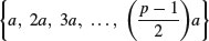
Lemma 2.3 (Gauss’s lemma) Let p be an odd prime number and suppose that . Further let be the number of integers in the set

whose least residues modulo p are negative, then

(2.144)

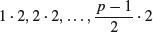
Proof: When we reduce the following numbers (modulo p)

to lie in set

then no two different numbers ma and na can go to the same numbers. Further, it cannot happen that ma goes to K and na goes to −k, because then , and hence (multiplying by the inverse of a), , which is impossible. Hence, when reducing the numbers

we get exactly one of −1 and 1, exactly one of −2 and 2, ..., exactly one of −(p−1)/2 and (p−1)/2. Hence, modulo p, we get

Cancelling the numbers , we have

By Euler’s criterion, we have Since , we must have .

Example 2.62 Use Gauss’s lemma to evaluate the Legendre symbol . By Gauss’s lemma, , where is the number of integers in the set

whose least residues modulo 11 are negative. Clearly,

So there are 3 least residues that are negative. Thus, . Therefore, . Consequently, the quadratic congruence is not solvable.

Remark 2.16 Gauss’s lemma is similar to Euler’s criterion in the following ways:

1. Gauss’s lemma provides a method for direct evaluation of the Legendre symbol;

2. It has more significance as a theoretical tool than as a computational tool.

Gauss’s lemma provides, among many other things, a means for deciding whether or not 2 is a quadratic residue modulo and odd prime p.

Theorem 2.68 If p is an odd prime, then

(2.145)

Proof: By Gauss’s lemma, we know that if is the number of least positive residues of the integers

that are greater than p/2, then . Let with . Then 2k<p/2 if and only if k<p/4; so [p/4] of the integers are less than p/2. So there are integers greater than p/2. Therefore, by Gauss’s lemma, we have

For the first equality, it suffices to show that

If , then p = 8k+1 for some , from which

and

so the desired congruence holds for . The cases for are similar. This completes the proof for the first equality of the theorem. Note that the cases above yield

which implies

This completes the second equality of the theorem.

Example 2.63 Evaluate and .

1. By Theorem 2.68, we have , since . Consequently, the quadratic congruence is solvable.

2. By Theorem 2.68, we have , since . Consequently, the quadratic congruence is not solvable.

Using Lemma 2.3, Gauss proved the following theorem, which is one of the great results of mathematics:

Theorem 2.69 (Quadratic reciprocity law) If p and q are distinct odd primes, then

1. if one of ;

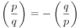2. if both .

Remark 2.17 This theorem may be stated equivalently in the form

(2.146)

Proof: We first observe that, by Gauss’s lemma, , where is the number of lattice points (x, y) (that is, pairs of integers) satisfying 0<x<q/2 and −q/2<px−qy<0. These inequalities give y<(px/q)+1/2<(p+1)/2. Hence, since y is an integer, we see is the number of lattice points in the rectangle r defined by 0<x<q/2, 0<y<p/2, satisfying −q/2<px−qy<0 (see Figure 2.2). Similarly, , where is the number of lattice points in r satisfying −p/2<qx−py<0. Now it suffices to prove that is even. But (p−1)(q−1)/4 is just the number of lattice points in r satisfying that or . The regions in r defined by these inequalities are disjoint and they contain the same number of lattice points, since the substitution

Figure 2.2 Proof of the quadratic reciprocity law

furnishes a one-to-one correspondence between them. The theorem follows.

Remark 2.18 The Quadratic Reciprocity Law was one of Gauss’s major contributions to mathematics. For those who consider number theory “the Queen of Mathematics,” this is one of the jewels in her crown. Since Gauss’s time, over 150 proofs of it have been published; Gauss himself published no less than six different proofs. Among the eminent mathematicians who contributed to the proofs are Cauchy, Jacobi, Dirichlet, Eisenstein, Kronecker, and Dedekind.

Combining all the above results for Legendre symbols, we get the following set of formulas for evaluating Legendre symbols:

(2.147)

(2.148)

(2.149)

(2.150)

(2.151)

(2.152)

(2.153)

(2.154)

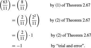
Example 2.64 Evaluate the Legendre symbol .

	by (2.150)
	by (2.151)
	by (2.152)
	by (2.149)
	by (2.153)

It follows that the quadratic congruence is soluble.

Example 2.65 Evaluate the Legendre symbol .

	by (2.151)
	by (2.153)
	by (2.154)
	by (2.150)
	by (2.151)
	by (2.152)
	by (2.153)

It follows that the quadratic congruence is not soluble.

Gauss’s Quadratic Reciprocity Law enables us to evaluate the values of Legendre symbols very quickly provided a is a prime or a product of primes, and p is an odd prime. However, when a is a composite, we must factor it into its prime factorization form in order to use Gauss’s quadratic reciprocity law. Unfortunately, there is no efficient algorithm so far for prime factorization (see Chapter 3 for more information). One way to overcome the difficulty of factoring a is to introduce the following Jacobi symbol (in honor of the German mathematician Carl Gustav Jacobi (1804–1851), which is a natural generalization of the Legendre symbol:

Definition 2.47 Let a be an integer and n>1 an odd positive integer. If , then the Jacobi symbol, , is defined by

(2.155)

where for is the Legendre symbol for the odd prime pi. If n is an odd prime, the Jacobi symbol is just the Legendre symbol.

The Jacobi symbol has some similar properties to the Legendre symbol, as shown in the following theorem.

Theorem 2.70 Let m and n be any positive odd composites, and . Then

1. If , then ;

2. ;

3. If , then ;

4. ;

5. ;

6. If , then .

Remark 2.19 It should be noted that the Jacobi symbol does not imply that a is a quadratic residue modulo n. Indeed a is a quadratic residue modulo n if and only if a is a quadratic residue modulo p for each prime divisor p of n. For example, the Jacobi symbol , but the quadratic congruence is actually not soluble. This is the significant difference between the Legendre symbol and the Jacobi symbol. However, does imply that a is a quadratic nonresidue modulo n. For example, the Jacobi symbol

and so we can conclude that 6 is a quadratic nonresidue modulo 35. In short, we have

(2.156)

Combining all the above results for Jacobi symbols, we get the following set of formulas for evaluating Jacobi symbols:

(2.157)

(2.158)

(2.159)

(2.160)

(2.161)

(2.162)

(2.163)

Example 2.66 Evaluate the Jacobi symbol .

	by (2.160)
	by (2.162)
	by (2.163)
	by (2.149)
	by (2.158)
	by (2.161)

It follows that the quadratic congruence is not soluble.

Example 2.67 Evaluate the Jacobi symbol .

	by (2.163)
	by (2.159)
	by (2.160)
	by (2.161)

Although the Jacobi symbol , we still cannot determine whether or not the quadratic congruence is soluble.

Remark 2.20 Jacobi symbols can be used to facilitate the calculation of Legendre symbols. In fact, Legendre symbols can be eventually calculated by Jacobi symbols. That is, the Legendre symbol can be calculated as if it were a Jacobi symbol. For example, consider the Legendre symbol , where is not a prime (of course, 2999 is prime, otherwise, it would not be a Legendre symbol). To evaluate this Legendre symbol, we first regard it as a Jacobi symbol and evaluate it as if it were a Jacobi symbol (note that once it is regarded as a Jacobi symbol, it does not matter whether or not 335 is prime; it even does not matter whether or not 2999 is prime, but anyway, it is a Legendre symbol).

Since 2999 is prime, is a Legendre symbol, and so 355 is a quadratic residue modulo 2999.

Table 2.4 Jacobi Symbols for

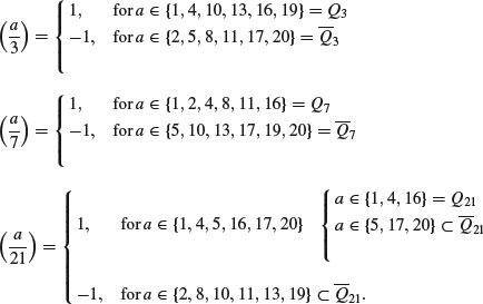
Example 2.68 In Table 2.4, we list the elements in and their Jacobi symbols. Incidentally, exactly half of the Legendre and Jacobi symbols , and are equal to 1 and half equal to −1. Also for those Jacobi symbols , exactly half of the a’s are indeed quadratic residues, whereas the other half are not. (Note that a is a quadratic residue of 21 if and only if it is a quadratic residue of both 3 and 7.) That is,

***************
browsing ---- left
******************

Problems for Section 2.4

1. Solve the following system of linear congruences:

2. Prove that n is prime if and

but

for each divisor m of n−1.

3. Show that the congruence

has just p−1 solutions modulo pk for every prime power pk.

4. Show that for any positive integer n, either there is no primitive root modulo n or there are primitive roots modulo n. (Note: Primitive roots are defined in Definition 2.49.)

5. Let d be the sum of all the distinct primitive roots modulo a prime p. Show that

6. Let n be a positive integer such that . Show that there are no integer solutions in x for

7. Show that for any prime p,

8. Suppose is prime. Show that

9. Let p be a prime. Show that for all positive integer , we have

Prove if , , , then

11. Find the x in and .

12. Compute the values for the Legendre symbol:

13. Which of the following congruences have solutions? If they have, then how many do they have?

14. Let p be a prime and . Prove that if , and are not soluble, then is soluble.

15. Prove that if p is a prime of the form 4k+1 then the sum of the quadratic residue modulo p in the interval [1, p) is p(p−1)/4.

16. Prove that if r is the quadratic residue modulo n>2, then

17. Let p, q be twin primes. Prove that there are infinitely many a such that if and only if there are infinitely many b such that

18. Prove that if and p an odd prime, then

19. Prove that if and p an odd prime, then

20. Let p be an odd prime, and let N++(p) be the number of n, such that

Prove that

2.5 Primitive Roots

Definition 2.48 Let n be a positive integer and a an integer such that . Then the order of a modulo n, denoted by ordn(a) or by ord(a, n), is the smallest integer r such that .

Remark 2.21 The terminology “the order of a modulo n” is the modern algebraic term from group theory (the theory of groups, rings, and fields will be formally introduced in Section 2.1). The older terminology “a belongs to the exponent r” is the classical term from number theory as used by Gauss.

Example 2.69 In Table 2.5, values of for are given.

From Table 2.5, we get

Table 2.5 Values of , for

We list in the following theorem some useful properties of the order of an integer a modulo n.

Theorem 2.71 Let n be a positive integer, , and r = ordn(a). Then

1. If , where m is a positive integer, then ;

2. ;

3. For integers s and t, if and only if ;

4. No two of the integers are congruent modulo r;

5. If m is a positive integer, then the order of am modulo n is ;

6. The order of am modulo n is r if and only if .

Definition 2.49 Let n be a positive integer and a an integer such that . If the order of an integer a modulo n is , that is, , then a is called a primitive root of n.

Example 2.70 Determine whether or not 7 is a primitive root of 45. First note that . Now observe that

	.

Thus, ord45(7) = 12. However, . That is, . Therefore, 7 is not a primitive root of 45.

Example 2.71 Determine whether or not 7 is a primitive root of 46. First note that . Now observe that

	.

Thus, ord46(7) = 22. Note also that . That is, . Therefore 7 is a primitive root of 46.

Theorem 2.72 (Primitive roots as residue system) Suppose . If G is a primitive root modulo n, then the set of integers is a reduced system of residues modulo n.

Example 2.72 Let n = 34. Then there are primitive roots of 34, namely, 3, 5, 7, 11, 23, 27, 29, 31. Now let g = 5 such that . Then

which forms a reduced system of residues modulo 34. We can of course choose g = 23 such that . Then we have

which again forms a reduced system of residues modulo 34.

Theorem 2.73 If p is a prime number, then there exist (incongruent) primitive roots modulo p.

Example 2.73 Let p = 47, then there are primitive roots modulo 47, namely,

Note that no method is known for predicting what will be the smallest primitive root of a given prime p, nor is there much known about the distribution of the primitive roots among the least residues modulo p.

Corollary 2.10 If n has a primitive root, then there are (incongruent) primitive roots modulo n.

Example 2.74 Let n = 46, then there are primitive roots modulo 46, namely,

Note that not all moduli n have primitive roots; in Table 2.6 we give the smallest primitive root G for that has primitive roots.

Table 2.6 Primitive roots G modulo n (if any) for

The following theorem establishes conditions for moduli to have primitive roots:

Theorem 2.74 An integer n>1 has a primitive root modulo n if and only if

(2.164)

where p is an odd prime and is a positive integer.

Corollary 2.11 If with , or with or , then there are no primitive roots modulo n.

Example 2.75 For n = 16 = 24, since it is of the form with , there are no primitive roots modulo 16.

Although we know which numbers possess primitive roots, it is not a simple matter to find these roots. Except for trial and error methods, very few general techniques are known. Artin in 1927 made the following conjecture (Rose [5]):

Conjecture 2.1 Let Na(x) be the number of primes less than x of which a is a primitive root, and suppose a is not a square and is not equal to −1, 0 or 1. Then

(2.165)

where a depends only on a.

Hooley in 1967 showed that if the extended Riemann Hypothesis is true then so is Artin’s conjecture. It is also interesting to note that before the age of computers Jacobi in 1839 listed all solutions of the congruences where , , G is the least positive primitive root of p and p<1000.

Another very important problem concerning the primitive roots of p is the estimate of the lower bound of the least positive primitive root of p. Let p be a prime and g(p) the least positive primitive root of p. The Chinese mathematician Yuan Wang [3] showed in 1959 that

1. ;

2. , if the Generalized Riemann Hypothesis (GRH) is true.

Wang’s second result was improved to by Victor Shoup [4] in 1992.

The concept of index of an integer modulo n was first introduced by Gauss in his Disquisitiones Arithmeticae. Given an integer n, if n has primitive root G, then the set

(2.166)

forms a reduced system of residues modulo n; G is a generator of the cyclic group of the reduced residues modulo n. (Clearly, the group is cyclic if , for p odd prime and positive integer.) Hence, if , then a can be expressed in the form:

(2.167)

for a suitable K with . This motivates our following definition, which is an analog of the real base logarithm function.

Definition 2.50 Let G be a primitive root of n. If , then the smallest positive integer K such that is called the index of a to the base G modulo n and is denoted by indg,n(a), or simply by indga.

Clearly, by definition, we have

(2.168)

The function indga is sometimes called the discrete logarithm and is denoted by logga so that

(2.169)

Generally, the discrete logarithm is a computationally intractable problem; no efficient algorithm has been found for computing discrete logarithms and hence it has important applications in public key cryptography.

Theorem 2.75 (Index theorem) If G is a primitive root modulo n, then if and only if .

Proof: Suppose that . Then, for some integer K. Therefore,

The proof of the “only if” part of the theorem is left as an exercise.

The properties of the function indga are very similar to those of the conventional real base logarithm function, as the following theorems indicate:

Theorem 2.76 Let G be a primitive root modulo the prime p, and . Then if and only if

(2.170)

Theorem 2.77 Let n be a positive integer with primitive root G, and . Then

1. ;

2. ;

3. , if K is a positive integer.

Example 2.76 Compute the index of 15 base 6 modulo 109, that is, . To find the index, we just successively perform the computation for until we find a suitable K such that :

	.

Since k = 20 is the smallest positive integer such that , .

In what follows, we shall study the congruences of the form , where n is an integer with primitive roots and . First of all, we present a definition, which is the generalization of quadratic residues.

Definition 2.51 Let a, n, and K be positive integers with . Suppose , then a is called a Kth (higher) power residue of n if there is an x such that

(2.171)

The set of all Kth (higher) power residues is denoted by K(k)n. If the congruence has no solution, then a is called a Kth (higher) power nonresidue of n. The set of such a is denoted by . For example, K(9)126 would denote the set of the 9th power residues of 126, whereas the set of the 5th power nonresidue of 31.

(2.172)

If 2.171 is soluble, then it has exactly gcd(k, (n)) incongruent solutions.

Proof: Let x be a solution of . Since , . Then

Conversely, if , then . Since , , and hence because must be an integer. Therefore, there are incongruent solutions to and hence incongruent solutions to .

If n is a prime number, say, p, then we have

Corollary 2.12 Suppose p is prime and . Then a is a Kth power residue of p if and only if

(2.173)

Example 2.77 Determine whether or not 5 is a sixth power of 31, that is, decide whether or not the congruence

has a solution. First of all, we compute

since 31 is prime. By Corollary 2.12, 5 is not a sixth power of 31. That is, . However,

So, 5 is a seventh power of 31. That is, .

Now let us introduce a new symbol , the Kth power residue symbol, analogous to the Legendre symbol for quadratic residues.

Definition 2.52 Let p be an odd prime, k>1, and . Then the symbol

(2.174)

is called the Kth power residue symbol modulo p, where represents the absolute smallest residue of modulo p. (The complete set of the absolute smallest residues modulo p are: ).

Theorem 2.79 Let be the Kth power residue symbol. Then

1. ;

2. ;

3. For ;

4. ;

5. a is the Kth power residue of ;

6. .

Example 2.78 Let p = 19, k = 3 and q = 6. Then

All the above congruences are modular 19.

Problems for Section 2.5

1. Find the primitive roots for primes 3, 5, 7, 11, 13, 17, 23.

2. Prove if and only if .

3. Show that the numbers form a reduced residue system modulo p if and only if .

4. Prove that if G and are primitive roots modulo an odd prime p, then is not a primitive root modulo p.

5. Let G be a primitive root modulo a prime p. Show that

Use this to prove the Wilson theorem:

6. Prove that if a and n>1 be any integers such that , but for every proper divisor d of n−1, then n is a prime.

7. For any positive integer n, prove that the arithmetic progression

contains infinitely many primes.

8. Show that if n>1, then .

9. Determine how many solutions each of the following congruence have.

10. (Victor Shoup) Let g(p) be the least positive primitive root modulo a prime p. Show that .

2.6 Elliptic Curves

The study of elliptic curves is intimately connected with the the study of Diophantine equations. The theory of Diophantine equations is a branch of number theory which deals with the solution of polynomial equations in either integers or rational numbers. As a solvable polynomial equation always has a corresponding geometrical diagram (e.g., curves or even surfaces). thus to find the integer or rational solution to a polynomial equation is equivalent to find the integer or rational points on the corresponding geometrical diagram, this leads naturally to Diophantine geometry, a subject dealing with the integer or rational points on curves or surfaces represented by polynomial equations. For example, in analytic geometry, the linear equation

(2.175)

represents a straight line. The points (x, y) in the plane whose coordinates x and y are integers are called lattice points. Solving the linear equation in integers is therefore equivalent to determining those lattice points that lie on the line; The integer points on this line give the solutions to the linear Diophantine equation ax+by+c = 0. The general form of the integral solutions for the equation shows that if (x0, y0) is a solution, then there are lattice points on the line:

(2.176)

If the polynomial equation is

(2.177)

then its associate algebraic curve is the unit circle. The solution (x, y) for which x and y are rational correspond to the Pythagorean triples x2+y2 = 1. In general, a polynomial f(x, y) of degree 2

(2.178)

gives either an ellipse, a parabola, or a hyperbola, depending on the values of the coefficients. If f(x, y) is a cubic polynomial in (x, y), then the locus of points satisfying f(x, y) = 0 is a cubic curve. A general cubic equation in two variables is of the form

(2.179)

Again, we are only interested in the integer solutions of the Diophantine equations, or equivalently, the integer points on the curves of the equations.

The above discussions lead us very naturally to Diophantine geometry, a subject dealing with the integer or rational points on algebraic curves or even surfaces of Diophantine equations (a straight line is a special case of algebraic curves).

Definition 2.53 A rational number, as everybody knows, is a quotient of two integers. A point in the (x, y)-plane is called a rational point if both its coordinates are rational numbers. A line is a rational line if the equation of the line can be written with rational numbers; that is, the equation is of the form

(2.180)

where a, b, c are rational numbers.

Definition 2.54 Let

(2.181)

be a conic. Then the conic is rational if we can write its equation with rational numbers.

We have already noted that the point of intersection of two rational lines is rational point. But what about the intersection of a rational line with a rational conic? Will it be true that the points of intersection are rational? In general, they are not. In fact, the two points of intersection are rational if and only if the roots of the quadratic equation are rational. However, if one of the points is rational, then so is the other.

There is a very general method to test, in a finite number of steps, whether or not a given rational conic has a rational point, due to Legendre. The method consists of determining whether a certain congruence can be satisfied.

Theorem 2.80 (Legendre) For the Diophantine equation

(2.182)

there is an integer n, depending on a, b, c, such that the equation has a solution in integers, not all zero, if and only if the congruence

(2.183)

has a solution in integers relatively prime to n.

An elliptic curve is an algebraic curve given by a cubic Diophantine equation

(2.184)

More general cubics in x and y can be reduced to this form, known as Weierstrass normal form, by rational transformations.

Example 2.79 Two examples of elliptic curves are shown in Figure 2.3 (from left to right). The graph on the left is the graph of a single equation, namely E1 : y2 = x3 - 4x + 2; even though it breaks apart into two pieces, we refer to it as a single curve. The graph on the right is given by the equation E2 : y2 = x3 - 3x + 3. Note that an elliptic curve is not an ellipse; a more accurate name for an elliptic curve, in terms of algebraic geometry, is an Abelian variety of dimension one. It should also be noted that quadratic polynomial equations are fairly well understood by mathematicians today, but cubic equations still pose enough difficulties to be topics of current research.

Figure 2.3 Two examples of elliptic curves

Definition 2.55 An elliptic curve E : y2 = x3+ax+b is called nonsingular if its discriminant

(2.185)

Remark 2.22 By elliptic curve, we always mean that the cubic curve is nonsingular. A cubic curve, such as y2 = x3−3x+2 for which , is actually not an elliptic curve; such a cubic curve with is called a singular curve. It can be shown that a cubic curve E : y2 = x3+ax+b is singular if and only if .

Definition 2.56 Let be a field. Then the characteristic of the field is 0 if

is never equal to 0 for any n>1. Otherwise, the characteristicof the field is the least positive integer n such that

Example 2.80 The fields , , , and all have characteristic 0, whereas the field is of characteristic p, where p is prime.

Definition 2.57 Let be a field (either the field , , , or the finite field with elements), and x3+ax+b with be a cubic polynomial. Then

1. If is a field of characteristic , then an elliptic curve over is the set of points (x, y) with that satisfy the following cubic Diophantine equation:

(2.186)

(where the cubic on the right-hand side has no multiple roots) together with a single element, denoted by , called the point at infinity.

2. If is a field of characteristic 2, then an elliptic curve over is the set of points (x, y) with that satisfy one of the following cubic Diophantine equations:

(2.187)

(here we do not care whether or not the cubic on the right-hand side has multiple roots) together with a point at infinity .

3. If is a field of characteristic 3, then an elliptic curve over is the set of points (x, y) with that satisfy the cubic Diophantine equation:

(2.188)

(where the cubic on the right-hand side has no multiple roots) together with a point at infinity .

In practice, we are actually more interested in the elliptic curves modulo a positive integer n.

Definition 2.58 Let n be a positive integer with . An elliptic curve over is given by the following cubic Diophantine equation:

(2.189)

where a, b and gcd(N, 4a3 + 27b2) = 1. The set of points on E is the set of solutions in to equation 2.189, together with a point at infinity .

Remark 2.23 The subject of elliptic curves is one of the jewels of 19th-century mathematics, originated by Abel, Gauss, Jacobi, and Legendre. Contrary to popular opinion, an elliptic curve (i.e., a nonsingular cubic curve) is not an ellipse; as Niven, Zuckerman, and Montgomery remarked, it is natural to express the arc length of an ellipse as an integral involving the square root of a quadratic polynomial. By making a rational change of variables, this may be reduced to an integral involving the square root of a cubic polynomial. In general, an integral involving the square root of a quadratic or cubic polynomial is called an elliptic integral. So, the word elliptic actually came from the theory of elliptic integrals of the form

(2.190)

where R(x, y) is a rational function in x and y, and y2 is a polynomial in x of degree 3 or 4 having no repeated roots. Such integrals were intensively studied in the 18th and 19th centuries. It is interesting to note that elliptic integrals serve as a motivation for the theory of elliptic functions, whilst elliptic functions parametrize elliptic curves. It is not our intention here to explain fully the theory of elliptic integrals and elliptic functions; interested readers are recommended to consult some more advanced texts.

The geometric interpretation of addition of points on an elliptic curve is quite straightforward. Suppose E is an elliptic curve as shown in Figure 2.4. A straight line L connecting points P and Q intersects the elliptic curve at a third point R, and the point is the reflection of R in the X-axis.

As can be seen from Figure 2.4, an elliptic curve can have many rational points; any straight line connecting two of them intersects a third. The point at infinity is the third point of intersection of any two points (not necessarily distinct) of a vertical line with the elliptic curve E. This makes it possible to generate all rational points out of just a few.

Figure 2.4 Geometric composition laws of an elliptic curve

The above observations lead naturally to the following geometric composition law of elliptic curves.

Proposition 2.3 (Geometric composition law (See 2.4)) Let P, Q E, L be the line connecting P and Q (tangent line to E if P = Q), and R be the third point of intersection of L with E. Let L′ be the line connecting R and (the point at infinity). Then is the point such that L′ intersects E at R, , and .

The points on an elliptic curve form an Abelian group with the addition of points as the binary operation on the group.

Theorem 2.81 (Group laws on elliptic curves) The geometric composition laws of elliptic curves have the following group-theoretic properties:

1. If a line L intersects e at the (not necessary distinct) points P, Q, R, then

2. .

3. .

4. Let , then there is a point of e, denoted , such that

5. Let , then

In other words, the composition law makes e into an Abelian group with identity element . We further have

6. Let e be defined over a field , then

is a subgroup of e.

Example 2.81 Let be the set of rational points on e. Then with the addition operation defined on it forms an Abelian group.

We shall now introduce the important concept of the order of a point on e.

Definition 2.59 Let p be an element of the set . Then p is said to have order K if

(2.191)

with for all (that is, K is the smallest integer such that ). If such a K exists, then p is said to have finite order, otherwise, it has infinite order.

Example 2.82 Let P = (3, 2) be a point on the elliptic curve E : y2 = x3−2x−3 over (see Example 2.87). Since and for k<10, p has order 10.

Example 2.83 Let P = (−2, 3) be a point on the elliptic curve E : y2 = x3+17 over (see Example 2.31). Then p apparently has infinite order.

Now let us move on to the problem as to how many points (rational or integral) are there on an elliptic curve? First let us look at an example:

Example 2.84 Let e be the elliptic curve y2 = x3+3x over , then

are the 10 points on e. However, the elliptic curve y2 = 3x3+2x over has only two points:

How many points are there on an elliptic curve E : y2 = x3+ax+b over ? The following theorem answers this question:

Theorem 2.82 Let with p prime be the number of points on E : y2 = x3+ax+b over . Then

(2.192)

points on E over , including the point at infinity , where is the Legendre symbol.

The quantity in (2.192) is constrained in the following theorem, due to Hasse (1898-1979) in 1933:

Theorem 2.83 (Hasse)

(2.193)

That is,

(2.194)

Example 2.84 Let p = 5, then . Hence, , that is,we have between 2 and 10 points on an elliptic curve over F5. In fact, all the possibilities occur in the elliptic curves given in Table 2.7.

Table 2.7 Number of points on elliptic curves over

A more general question is: How many rational points are there on an elliptic curve E : y2 = x3+ax+b over ? Louis Joel Mordell (1888–1972) solved this problem in 1922:

Theorem 2.84 (Mordell’s finite basis theorem) Suppose that the cubic polynomial f(x, y) has rational coefficients, and that the equation f(x, y) = 0 defines an elliptic curve e. Then the group of rational points on e is a finitely generated Abelian group.

In elementary language, this says that on any elliptic curve that contains a rational point, there exists a finite collection of rational points such that all other rational points can be generated by using the chord-and-tangent method. From a group-theoretic point of view, Mordell’s theorem tells us that we can produce all of the rational points on e by starting from some finite set and using the group laws. It should be noted that for some cubic curves, we have tools to find this generating set, but unfortunately, there is no general method (i.e., algorithm) guaranteed to work for all cubic curves.

The fact that the Abelian group is finitely generated means that it consists of a finite “torsion subgroup” Etors, consisting of the rational points of finite order, plus the subgroup generated by a finite number of points of infinite order:

The number r of generators needed for the infinite part is called the rank of ; it is zero if and only if the entire group of rational points is finite. The study of the rank r and other features of the group of points on an elliptic curve over are related to many interesting problems in number theory and arithmetic algebraic geometry. One of such problems is the Birch and Swinerton-Dyer conjecture (BSD conjecture), which shall be dicussed later.

The most important and fundamental operation on an elliptic curve is the addition of points on the curve. To perform the addition of points on elliptic curves systematically, we need an algebraic formula. The following gives us a convenient computation formula.

Theorem 2.85 (Algebraic computation law) Let P1 = (x1, y1), P2 = (x2, y2) be points on the elliptic curve:

(2.195)

then on e may be computed by

(2.196)

where

(2.197)

and

(2.198)

Example 2.86 Let e be the elliptic curve y2 = x3+17 over , and let P1 = (x1, y1) = (−2, 3) and P2 = (x2, y2) = (1/4,  33/8) be two points on e. To find the third point P3 on e, we perform the following computation:

So .

Example 2.87 Let P = (3, 2) be a point on the elliptic curve E : y2 = x3−2x−3 over . Compute

According to (2.197), we have:

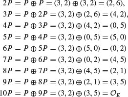
Example 2.88 Let E : y2 = x3+17 be the elliptic curve over and P = (−2, 3) a point on e. Then

Suppose now we are interested in measuring the size (or the height of point on elliptic curve) of points on an elliptic curve e. One way to do this is to look at the numerator and denominator of the x-coordinates. If we write the coordinates of as

(2.199)

we may define the height of these points as follows

(2.200)

It is interesting to note that for large K, the height of looks like:

(2.201)

(2.202)

where denotes the number of digits in .

Remark 2.24 To provide greater flexibility, we may also consider the following form of elliptic curves:

(2.203)

In order for e to be an elliptic curve, it is necessary and sufficient that

(2.204)

Thus,

on e may be computed by

(2.205)

where

(2.206)

The problem of determining the group of rational points on an elliptic curve E : y2 = x3+ax+b over , denoted by , is one of the oldest and most intractable in mathematics, and it remains unsolved to this day, although vast numerical evidences exist. In 1922, Louis Joel Mordell (1888–1972) showed that is a finitely generated (Abelian) group. That is, where , is a finite Abelian group (called torsion group). The integer r is called the rank of the elliptic curve E over , denoted by . Is there an algorithm to compute given an arbitrary elliptic curve E? The answer is not known, although can be found easily, due to a theorem of Mazur in 1978: . The famous Birch and Swinnerton-Dyer conjecture [6], or BSD conjecture for short, asserts that the size of the group of rational points on E over , denoted by , is related to the behavior of an associated zeta function , called the Hasse–Weil L-function L(E, s), near the point s = 1. That is, if we define the incomplete L-function L(E, s) (we called it incomplete because we omit the set of “bad” primes ) as follows:

where is the discriminant of e, with p prime and ap = p−Np. This L-function converges for , and can be analytically continued to an entire function. It was conjectured by Birch and Swinnerton-Dyer in the 1960s that the rank of the Abelian group of points over a number field of an elliptic curve e is related to the order of the zero of the associated L-function L(E, s) at s = 1:

BSD Conjecture (Version 1):

This amazing conjecture asserts particularly that

Conversely, if , then the set is finite. An alternative version of BSD, in term of the Taylor expansion of L(E, s) at s = 1, is as follows:

BSD Conjecture (Version 2): where and .

There is also a refined version of BSD for the complete L-function :

In this case, we have:

BSD Conjecture (Version 3): with

where |IIIE| is the order of the Tate–Shafarevich group of elliptic curve e, the term is an determinant whose matrix entries are given by a height pairing applied to a system of generators of , the wp are elementary local factors and is a simple multiple of the real period of e.

The eminent American mathematician, John Tate commented on BSD in 1974 that “… this remarkable conjecture relates the behaviour of a function L at a point where it is at present not known to be defined to the order of a group III which is not known to be finite.” So it was hoped that a proof of the conjecture would yield a proof of the finiteness of IIIE. Using the idea of Kurt Heegner (1893–1965), Birch and his former PhD student Stephens established for the first time the existence of rational points of infinite order on certain elliptic curves over , without actually writing down the coordinates of these points, and naively verifying that they had satisfied the equation of the curves. These points are now called Heegner points on elliptic curves (a Heegner point is a point on modular elliptic curves that is the image of a quadratic imaginary point of the upper half-plane). Based on Birch and Stephens’ work, particular on their massive computation of the Heegner points on modular elliptic curves, Gross at Harvard and Zagier at Maryland/Bonn obtained a deep result in 1986, now widely known as the Gross–Zagier theorem, which describes the height of Heegner points in terms of a derivative of the L-function of the elliptic curve at the point s = 1. That is, if L(E, 1) = 0, then there is a closed formula to relate L′(E,1) and the height of the Heegner points on E. More generally, together with Kohnen, Gross and Zagier showed in 1987 that Heegner points could be used to construct rational points on the curve for each positive integer n, and the heights of these points were the coefficients of a modular form of weight 3/2. Later, in 1989, the Russian mathematician Kolyvagin further used Heegner points to construct Euler systems, and used this to prove much of the Birch–Swinnerton-Dyer conjecture for rank 1 elliptic curves. More specifically, he showed that if the Heegner points are of infinite order, then . Other notable results in BSD also include S. W. Zhang’s generalization of Gross–Zagier theorem for elliptic curves to Abelian varieties, and M. L. Brown’s proof of BSD for most rank 1 elliptic curves over global fields of positive characteristic. Of course, all these resolutions are far away from the complete settlement of BSD. Just as Riemann’s Hypothesis, the BSD conjecture was also chosen to be one of the seven Millennium Prize Problems [7].

Problems for Section 2.6

1. Describe an algorithm to find a point on an elliptic curve E : y2 = x3+ax+b over . Use your algorithm to find a point on the E : y2 = x3−13x+21 over .

2. Find all the rational points on the elliptic curve y2 = x3−x.

3. Find all the rational points on the elliptic curve y2 = x3+4x.

4. Describe an algorithm to find the order of a point on an elliptic curve E : y2 = x3+ax+b over . Let P = (2, 4) be a point on E : y2 = x3−13x+21 over . Use your algorithm to find the order of the point on e.

5. Find all the torsion points of the elliptic curve E : y2 = x3−13x+21 over .

6. Find the point of infinite order on the elliptic curve E : y2 = x3−2x over .

7. Determine the number of points of the elliptic curve E : y2 = x3−1 for all odd primes up to 100.

8. Let P = (0, 0) be a point on the elliptic curve E : y2 = x3+x2+2x. Compute 100P and 200P.

9. Derive an addition formula for rational points on the elliptic curve

10. Show that P = (9/4, 29/8) is a point on the elliptic curve E : y2 = x3−x+4.

11. Let P = (1, 1) be a point on the elliptic curve E : y2 = x3−6x+6 over . Compute 100P on .

12. Let n be a positive integers greater than 1, and p a point on an elliptic curve . Prove that there are some integers s and t such that sP = tP.

13. Prove or disprove the BSD conjecture.

2.7 Bibliographic Notes and Further Reading

This chapter was mainly concerned with the elementary theory of numbers, including Euclid’s algorithm, continued fractions, the Chinese Remainder theorem, Diophantine equations, arithmetic functions, quadratic and power residues, primitive roots, and the arithmetic of elliptic curves. It also includes some algebraic topics such as groups, rings, fields, polynomials, and algebraic numbers. The theory of numbers is one of the oldest and most beautiful parts of pure mathematics, and there are many good books and papers in this field.

It is suggested that readers consult some of the following references for more information: [8-28].

Elliptic curves are used throughout the book for primality testing, integer factorization, and cryptography. We have only given an brief introduction to the theory and arithmetic of elliptic curves. Readers who are interested in elliptic curves and their applications should consult the following references for more information: [29-33]. Also, the new version of Hardy and E. M. Wright’s famous book [14] also contains a new chapter on elliptic curves at the end of the book.

Abstract algebra is intimately connected to number theory and, in fact, many of the concepts and results of number theory can be described in algebraic language. Readers who wish to study number theory from the algebraic perspective are specifically advised to consult the following references: [34-48].

References

1. G. E. Andrews, Number Theory, W. B. Sayders Company, 1971. Also Dover Publications, 1994.

2. H. Davenport, The Higher Arithmetic, 7th Edition, Cambridge University Press, 1999.

3. Y. Wang, “On the Least Positive Primitive Root”, The Chinese Journal of Mathematics, 9, 4, 1959, pp. 432–441.

4. V. Shoup, “Searching for Primitive Roots in Finite Fields”, Mathematics of Computation, 58, 197, 1992, pp. 369–380.

5. H. E. Rose, A Course in Number Theory, 2nd Edition, Oxford University Press, 1994.

6. A. Wiles, “The Birch and Swinnerton-Dyer Conjecture”, In [7]: The Millennium Prize Problems, American Mathematical Society, 2006, pp. 31–44.

7. J. Carlson, A. Jaffe, and A. Wiles, The Millennium Prize Problems, Clay Mathematics Institute and American Mathematical Society, 2006.

8. A. Baker, A Concise Introduction to the Theory of Numbers, Cambridge University Press, 1984.

9. E. D. Bolker, Elementray Number Theory: An Algebraic Approach, Dover, 2007.

10. D. M. Burton, Elementary Number Theory, 7th Edition, McGraw-Hill, 2011.

11. H. Davenport, The Higher Arithmetic, 7th Edition, Cambridge University Press, 1999.

12. U. Dudley, A Guide to Elementary Number Theory, Mathematical Association of America, 2010.

13. H. M. Edwards, Higher Arithmetic: Al Algorithmic Introduction to Number Theory, American Mathematical Society, 2008.

14. G. H. Hardy and E. M. Wright, An Introduction to Theory of Numbers, 6th Edition, Oxford University Press, 2008.

15. L.K. Hua, Introduction to Number Theory, Springer, 1980.

16. K. Ireland and M. Rosen, A Classical Introduction to Modern Number Theory, 2nd Edition, Graduate Texts in Mathematics 84, Springer, 1990.

17. N. Koblitz, A Course in Number Theory and Cryptography, 2nd Edition, Graduate Texts in Mathematics 114, Springer, 1994.

18. W. J. LeVeque, Fundamentals of Number Theory, Dover, 1977.

19. S. J. Miller and R. Takloo-Bighash, An Invitation to Modern Number Theory, Princeton University Press, 2006.

20. R. A. Mollin, Fundamental Number Theory with Applications, 2nd Edition, CRC Press, 2008.

21. R. A. Mollin, Advanced Number Theory with Applications, CRC Press, 2010.

22. R. A. Mollin, Algebraic Number Theory, 2nd Edition, CRC Press, 2011.

23. I. Niven, H. S. Zuckerman, and H. L. Montgomery, An Introduction to the Theory of Numbers, 5th Edition, John Wiley & Sons, 1991.

24. J. E. Pommersheim, T. K. Marks, and E. L. Flapan, Number Theory, Wiley, 2010.

25. J. E. Shockley, Introduction to Number Theory, Holt, Rinehart and Winston, 1967.

26. J. H. Silverman, A Friendly Introduction to Number Theory, 4th Edition, Prentice-Hall, 2012.

27. J. Stillwell, Elements of Number Theory, Springer, 2000.

28. S. Y. Yan, Number Theory for Computing, 2nd Edition, Springer, 2002.

29. A. Ash and R. Gross, Elliptic Tales: Curves, Counting, and Number Theory, Princeton University Press, 2012.

30. D. Husemöller, Elliptic Curves, Graduate Texts in Mathematics 111, Springer, 1987.

31. J. H. Silverman, The Arithmetic of Elliptic Curves, 2nd Edition, Graduate Texts in Mathematics 106, Springer, 2009.

32. J. H. Silverman and J. Tate, Rational Points on Elliptic Curves, Undergraduate Texts in Mathematics, Springer, 1992.

33. L. C. Washinton, Elliptic Curve: Number Theory and Cryptography, 2nd Edition, CRC Press, 2008.

34. M. Artin, Algebra, 2nd Edition, Prentice-Hall, 2011.

35. P. E. Bland, The Basics of Abstract Algebra, W. H. Freeman and Company, 2002.

36. L. N. Childs, A Concrete Introduction to Higher Algebra, 3rd Edition, Springer, 2009.

37. J. B. Fraleigh, First Course in Abstract Algebra, 7th Edition, Addison-Wesley, 2003.

38. J. A. Gallian, Contemporary Abstract Algebra, 5th Edition, Houghton Mifflin Company, 2002.

39. D. W. Hardy, F. Richman, and C. L. Walker, Applied Algebra, 2nd Edition, Addison-Wesley, 2009.

40. I. N. Herstein, Abstract Algebra, 3rd Edition, Wiley, 1999.

41. T. W. Hungerford, Abstract Algebra: An Introduction, 2nd Edition, Brooks/Cole, 1997.

42. S. Lang, Algebra, 3rd Edition, Springer, 2002.

43. R. Lidl and G. Pilz, Applied Abstract Algebra, Springer, 1984.

44. S. MacLane and G. Birkhoff, Algebra, 3rd Edition, AMS Chelsea, 1992.

45. G. L. Mullen and C. Mummert, Finite Fields and Applications, Mathematical Association of America, 2007.

46. J. J. Rotman, A First Course in Abstract Algebra, 3rd Edition, Wiley, 2006.

47. V. Shoup, A Computational Introduction to Number Theory and Algebra, Cambridge University Press, 2005.

48. J. Stillwell, Elements of Algebra, Springer, 1994.

1. The order of an element a modulo n is the smallest integer r such that ; we shall discuss this later in Section 2.5.