3

Primality Testing

Primality testing, possibly first studied by Euclid 2500 years ago but first identified as an important problem by Gauss in 1801, is one of the two important problems related to the computation of prime numbers. In this chapter we shall study various modern algorithms for primality testing, including

• Some simple and basic tests of primality, usually run in exponential-time .
• The Miller–Rabin test, runs in random polynomial-time .
• The elliptic curve test, runs in zero-error probabilistic polynomial-time .
• The AKS test, runs in deterministic polynomial-time .

3.1 Basic Tests

The Primality Test Problem (PTP) may be described as follows:

(3.1)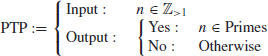

The following theorem is well-known and fundamental to primality testing.

Theorem 3.1 Let n>1. If n has no prime factor less than or equal to , then n is prime.

Thus the simplest possible primality test of n is by trial divisions of all possible prime factors of n up to as follows (the Sieve of Eratosthenes for finding all prime numbers up to is used in this test).

Primality test by trial divisions:

(3.2)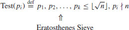

Thus, if n passes Test(pi), then n is prime:

(3.3)

Example 3.1 To test whether or not 3271 is prime, we only need to test the primes up to 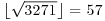. That is, we will only need to do at most 16 trial divisions as follows:

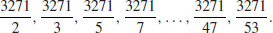
As none of these division gives a zero remainder, so 3271 is a prime number. However, for n = 3273, we would normally expect to do the following trial divisions:

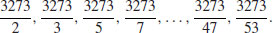
but fortunately we do not need to do all these trial divisions as 3273 is a composite, in fact, when we do the trial division 3273/3, it gives a zero remainder, so we conclude immediately that 3273 is a composite number.

This test, although easy to implement, is not practically useful for large numbers since it needs bit operations. In other words, it runs in exponential-time, . In the next sections, we shall introduce some modern and fast primality testing methods in current use. From a computational complexity point of view, the PTP has been completely solved since we have various algorithms for PTP, with the fastest runs in deterministic polynomial-time (see Figure 3.1).

In 1876 (although it was published in 1891), Lucas discovered a type of converse of the Fermat little theorem, based on the use of primitive roots.

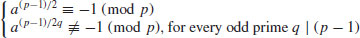
Theorem 3.2 (Lucas’ converse of Fermat’s little theorem, 1876) Let n>1. Assume that there exists a primitive root of n, i.e., an integer a such that

1. ,

2. , for each prime divisor p of n−1.

Then n is prime.

Proof: Since , Part (1) of Theorem 2.71 (see Chapter 1) tells us that . We will show that ordn(a) = n−1. Suppose . Since (n−1), there is an integer k satisfying . Since , we know that k>1. Let p be a prime factor of k. Then

However, this contradicts the hypothesis of the theorem, so we must have ordn(a) = n−1. Now, since and , it follows that . So finally by Part (2) of Theorem 2.36, n must be prime.

Lucas’ theorem can be converted to rigorous primality test as follows:

Primality test based on primitive roots:

(3.4)

If n passes the test, then n is prime:

(3.5)

Primality test based on primitive roots is also called n−1 primality test, as it is based on the prime factorization of n−1.

Example 3.2 Let n = 2011, then . Note first 3 is a primitive root (in fact, the smallest) primitive root of 2011, since . So, we have

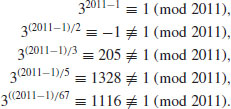
Thus, by Theorem 3.2, 2011 must be prime.

Remark 3.1 In practice, primitive roots tend to be small integers and can be quickly found (although there are some primes with arbitrary large smallest primitive roots), and the computation for and can also be performed very efficiently. However, to determine if n is prime, the above test requires the prime factorization of n−1, a problem of almost the same size as that of factoring n, and a problem that is much harder than the primality testing of n.

Note that Theorem 3.2 is actually equivalent to the following theorem:

Theorem 3.3 If there is an integer a for which the order of a modulo n is equal to and , then n is prime. That is, if

(3.6)

or

(3.7)

then n is prime.

Thus, we have the following primality test.

Primality test based on ordn(a)

(3.8)

Thus, if n passes the test, then n is prime:

(3.9)

Example 3.3 Let n = 3779. We find, for example, that the integer a = 19 with satisfies

1. ord3779(19) = 3778,

2. .

That is, . Thus by Theorem 3.3, 3779 is prime.

Remark 3.2 It is not a simple matter to find the order of an element a modulo n, ordn(a), if n is large. In fact, if ordn(a) can be calculated efficiently, the primality and prime factorization of n can be easily determined. At present, the best known method for computing ordn(a) requires one to factor n.

Remark 3.3 If we know the value of , we can immediately determine whether or not n is prime, since by Part (2) of Theorem 2.36 we know that n is prime if and only if . Of course, this method is not practically useful, since to determine the primality of n, we need to find , but to find , we need to factor n, a problem even harder than the primality testing of n.

Remark 3.4 The difficulty in applying Theorem 3.3 for primality testing lies in finding the order of an integer a modulo n, which is computationally intractable. As we will show later, the finding of the order of an integer a modulo n can be efficiently done on a quantum computer.

It is possible to use different bases ai (rather than a single base a) for different prime factors pi of n−1 in Theorem 3.2:

Theorem 3.4 If for each prime pi of n−1 there exists an integer ai such that

1. ,

2. .

Then n is prime.

Proof: Suppose that , with , for . Let also ri = ordn(ai). Then and gives that . But for each i, we have and hence . This gives , so n must be prime.

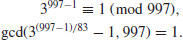
Example 3.4 Let n = 997, then . We choose three different bases 5, 7, 11 for the prime factors 2, 3, 83, respectively, and get

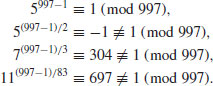
Thus, we can conclude that 997 is prime.

The above tests require the factorization of n−1, a problem even harder than the primality test of n. In 1914, Henry C. Pocklington (1870–1952) showed that it is not necessary to know all the prime factors of n−1; part of them will be sufficient, as indicated in the following theorem.

Theorem 3.5 (Pocklington, 1914) Let n−1 = mj, with , , and . If for each prime , there exists an integer a such that

1. ,

2. .

Then n is prime.

Proof: Let q be any one of the prime factors of n, and ordn(a) the order of a modulo n. We have and also , but . Hence, . Since , the result thus follows.

As already pointed out by Pocklington, the above theorem can lead to a primality test:

Pocklington’s Test

(3.10)

Thus, if n passes the test, then n is prime:

(3.11)

Example 3.5 Let also n = 997, and , . Choose a = 3 for m = 83. Then we have

Thus, we can conclude that 997 is prime.

There are some other rigorous, although inefficient, primality tests, for example one of them follows directly from the converse of Wilson’s theorem (Theorem 2.59)

Wilson’s test

(3.12)

Thus, if n passes the test, then n is prime:

(3.13)

Remark 3.5 Unfortunately, very few primes satisfy the condition, in fact, for , there are only three primes, namely, p = 5, 13, 563. So the Wilson test is essentially of no use in primality testing, not just because of its inefficiency.

Pratt’s primality proving

It is interesting to note that, although primality testing is difficult, the verification (proving) of primality is easy, since the primality (as well as the compositeness) of an integer n can be verified very quickly in polynomial-time:

Theorem 3.6 If n is composite, it can be proved to be composite in bit operations.

Proof: If n is composite, there are integers a and b with 1<a<n, 1<b<n and n = ab. Hence, given the two integers a and b, we multiply a and b, and verify that n = ab. This takes bit operations and proves that n is composite.

Theorem 3.7 If n is prime, then it can be proved to be prime in bit operations.

Figure 3.1 Algorithms/Methods for PTP

Figure 3.2 Certificate of primality for n = 2557

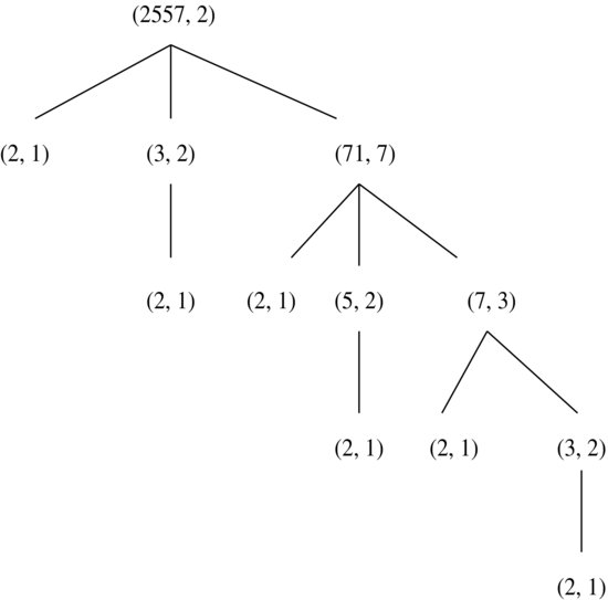
Theorem 3.7 was discovered by Pratt [3] in 1975; he interpreted the result as showing that every prime has a succinct primality certification. The proof can be written as a finite tree whose vertices are labeled by pairs (p, gp) where p is a prime number and gp is primitive root modulo p; we illustrate the primality proving of prime number 2557 in Figure 3.2. In the top level of the tree, we write (2557, 2) with 2 the primitive root modulo 2557. As , we have in the second level three vertices (2, 1), (3, 2), (71, 7). Since 3, 71>2, we have in the third level the child vertices (2, 1) for (3, 2), (2, 1), (5, 2) ,and (7, 3) for (71, 7). In the fourth level of the tree, we have (2, 1) for (5, 2), (2, 1) and (3, 2) for (7, 3). Finally, in the fifth level we have (2, 1) for (3, 2). The leaves of the tree now are all labeled (2, 1), completing the certification of the primality of 2557.

Remark 3.6 It should be noted that Theorem 3.7 cannot be used for finding the short proof of primality, since the factorization of n−1 and the primitive root a of n are required.

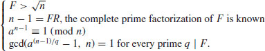
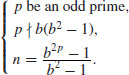
Note that for some primes, Pratt’s certificate is considerably shorter. For example, if is a Fermat number with , the p is prime if and only if

(3.14)

This result, known as Papin’s test, gives a Pratt certificate for Fermat primes. The work in verifying (3.14) is just , since . In fact, it can be shown that every prime p has an certificate. More precisely, we can have:

Theorem 3.8 For every prime p there is a proof that it is prime which requires for its certification (5/2 + o(1))log2p multiplications modulo p.

Problems for Section 3.1

1. Use the Primality test based on primitive roots defined in (3.4) to prove that 1299709 is prime (choose a = 6).

2. Use the primality test based on Pocklington’s theorem defined in (3.10) to prove that 179424673 is prime.

3. Prove that if p>1 is an odd integer and

(3.15)

Then p is prime. Conversely, if p is an odd prime, then every primitive root a of p satisfies conditions (3.15).

4. Prove or disprove that there are infinitely many Wilson primes (i.e., those primes p satisfying the condition ).

5. Prove that if

Then p is prime.

6. (Brillhart, Lehmer, and Selfridge). Suppose

Represent a as a base F form n = c2F2 + c1F + 1, where . Show that p is prime if and only if c21−4c2 is not a square.

7. (Proth, 1878). Let n = 2km + 1, with , 2k>m, and suppose that . Then n is prime if and only if

8. Use Proth’s result to prove that the following three numbers are prime:

9. (Pocklington, 1914). Let n = pkm + 1, with p prime and , Show that if for some a we have

(3.16)

then each prime factor of n is of the form spk + 1 for some s.

10. Use the Pratt tree to prove the primality of 123456791.

11. Show that for any positive integer n>4, the following three statements are equivalent:

1. n is composite,

2. ,

3. .

12. Let

Then n is a based b pseudoprime.

3.2 Miller–Rabin Test

The Miller–Rabin test[1, 2], also known as the strong pseudoprimality test, or more precisely, the Miller–Selfridge–Rabin test, is a fast and practical probabilistic primality test; its probabilistic error can be reduced to as small as we desire, but not to zero. In terms of computational complexity, it runs in . The test is also some times called strong pseudoprimality test. The test was first studied by Miller in 1976 and Rabin in 1980, but was used by Selfridge in 1974, even before Miller and Rabin published their result.

Theorem 3.9 Let p be a prime. Then

(3.17)

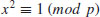
if and only if .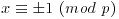

Proof: First notice that

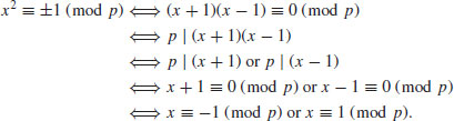
Conversely, if either or holds, then .   

Definition 3.1 The number x is called a nontrivial square root of 1 modulo n if it satisfies (3.17) but .

Example 3.6 The number 6 is a nontrivial square root of 1 modulo 35. Since , .

Corollary 3.1 If there exists a nontrivial square root of 1 modulo n, then n is composite.

Example 3.7 Show that 1387 is composite. Let x = 2693. We have , but . So, 2693 is a nontrivial square root of 1 modulo 1387. Then by Corollary 72, 1387 is composite.

Theorem 3.10 (Miller–Rabin Test) Let n be an odd prime number: n = 1 + 2jd, with d odd. Then the b-sequence defined by

(3.18)

has one of the following two forms:

(3.19)

(3.20)

reduced to modulo n, for any 1 < b < n. (The question mark “?” denotes a number different from ± 1.)

The correctness of the above theorem relies on Theorem 3.9: If n is prime, then the only solutions to are . To use the strong pseudoprimality test on n, we first choose a base b, usually a small prime. Then compute the b-sequence of n; write n−1 as 2jd where d is odd, compute , the first term of the b-sequence, and then square repeatedly to obtain the b-sequence of j + 1 numbers defined in (3.18), all reduced to modulo n. If n is prime, then the b-sequence of n will be of the form of either (3.19) or (3.20). If the b-sequence of n has any one of the following three forms

(3.21)

(3.22)

(3.23)

then n is certainly composite. However, a composite can masquerade as a prime for a few choices of base b, but should not be “too many.” The above idea leads naturally to a very efficient and also a practically useful algorithm for (pseudo) primality testing:

Algorithm 3.1 (Miller–Rabin test) This algorithm will test n for primality with high probability:

1. Let n be an odd number, and the base b a random number in the range 1<b<n. Find j and d with d odd, so that n−1 = 2jd.

2. Set and .

3. If i = 0 and y = 1, or y = n−1, then terminate the algorithm and output “n is probably prime.” If i>0 and y = 1 go to [5].

4. . If i<j, set and return to [3].

5. Terminate the algorithm and output “n is definitely not prime.”

Theorem 3.11 The strong pseudoprimality test above runs in time .

Definition 3.2 A positive integer n with and d odd, is called a base-b strong probable prime if it passes the strong pseudoprimality test described above (i.e., the last term in sequence (3.18) is 1, and the first occurrence of 1 is either the first term or is preceded by −1). A base-b strong probable prime is called a base-b strong pseudoprime if it is a composite.

If n is prime and 1<b<n, then n passes the test. The converse is usually true, as shown by the following theorem.

Theorem 3.12 Let n>1 be an odd composite integer. Then n passes the strong test for at most (n−1)/4 bases b with .

Proof: The proof is rather lengthy, we thus only give a sketch of the proof. A more detailed proof can be found either in Section 8.4 of Rosen [44], or in Chapter V of Koblitz [37]. First note that if p is an odd prime, and and q are positive integers, then the number of incongruent solutions of the congruence

is . Let , where d is an odd positive integer and j is a positive integer. For n to be a strong pseudoprime to the base b, either

or

for some integer i with 0<i<j−1. In either case, we have

Let the standard prime factorization of n be

By the assertion made at the beginning of the proof, we know that there are

incongruent solutions to the congruence

Further, by the Chinese Remainder theorem, we know that there are exactly

incongruent solutions to the congruence

To prove the theorem, there are three cases to consider:

1. the standard prime factorization of n contains a prime power with exponent ;

2. n = pq, with p and q distinct odd primes;

3. n = p1p2···pk, with distinct odd primes.

The second case can actually be included in the third case. We consider here only the first case. Since

we have

Thus, there are at most (n−1)/4 integers b, 1<b<n−1, for which n is a base-b strong pseudoprime and n can pass the strong test.

A probabilistic interpretation of Theorem 3.12 is as follows:

Corollary 3.2 Let n>1 be an odd composite integer and b be chosen randomly from . Then the probability that n passes the strong test is less than 1/4.

From Corollary 3.2, we can construct a simple, general purpose, polynomial time primality test which has a positive (but arbitrarily small) probability of giving the wrong answer. Suppose an error probability of is acceptable. Choose k such that , and select randomly and independently from . If n fails the strong test on bi, , then n is a strong probable prime.

Theorem 3.13 The strong test (i.e., Algorithm 3.1) requires, for n−1 = 2jd with d odd and for k randomly selected bases, at most k(2 + j)log n steps. If n is prime, then the result is always correct. If n is composite, then the probability that n passes all k tests is at most 1/4k.

Proof: The first two statements are obvious, only the last statement requires proof. An error will occur only when the n to be tested is composite and the bases chosen in this particular run of the algorithm are all nonwitnesses. (An integer a is a witness to the compositeness of n if it is possible using a to prove that n is composite, otherwise it is a nonwitness). Since the probability of randomly selecting a nonwitness is smaller than 1/4 (by Corollary 3.2), then the probability of independently selecting k nonwitnesses is smaller than 1/4k. Thus the probability that with any given number n, a particular run of the algorithm will produce an erroneous answer is smaller than 1/4k [2].

Problems for Section 3.2

1. Show that there are infinitely many base 2 strong pseudoprime numbers.

2. Show that there are infinitely many base b strong pseudoprime numbers.

3. Show that there are infinitely many base 2 Euler pseudoprime numbers.

4. Show that there are infinitely many base b Euler pseudoprime numbers.

5. Show that if n is an odd composite number, then there exists an integer b such that and n is not a base b Euler pseudoprime.

6. Show that if n is a base b strong pseudoprime, then n is also a base b Euler pseudoprime.

7. Let n>1 be an odd integer. Show that n is prime if and only if

8. Let n>1 be an odd integer. Show that n is prime if and only if

9. Let Rn be the set

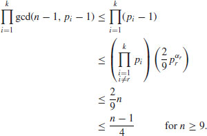
where n−1 = 2ku, u odd, and is restricted to . Prove that for all odd composite integer n>9,

10. Prove the following theorem: Let n = FR + 1, where 0<R<F. If for some a we have

Then n is a prime.

11. Prove Selfridge’s theorem: Let n>1 be an odd integer. If

where are primes and each pi there exists an ai such that

Then n is a prime.

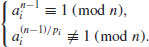
3.3 Elliptic Curve Tests

In the last 20 years or so, there have been some surprising applications of elliptic curves to problems in primality testing, integer factorization and public-key cryptography. In 1985, Lenstra [4] announced an elliptic curve factoring method (the formal publication was in 1987), just one year later, Goldwasser and Kilian in 1986 [5] adapted Lenstra’s factoring algorithm to obtain an elliptic curve primality test, and Miller in 1986 [6] and Koblitz in 1987 [7] independently arrived at the idea of elliptic curve cryptography. In this section, we discuss fast primality tests based elliptic curves. These tests, though, are still probabilistic, with zero error. In terms of computational complexity, they run in .

First we introduce a test based on Cox in 1989 [8].

Theorem 3.14 (Cox) Let with n>13 and , and let be an elliptic curve over . Suppose that

1. .

2. , with q an odd prime.

If is a point on E and , then n is prime.

Proof: See pp. 324–325 of Cox in 1989 [8].

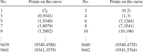
Example 3.8 Suppose we wish to prove that n = 9343 is a prime using the above elliptic curve test. First notice that n>13 and . Next, we choose an elliptic curve y2 = x3 + 4x + 4 over with P = (0, 2), and calculate , the number of points on the elliptic curve , Suppose we use the numerical exhaustive method, we then know that there are 9442 points on this curve:

Thus, 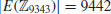. Now we are ready to verify the two conditions in Theorem 3.14. For the first condition, we have:

For the second condition, we have:

So, both conditions are satisfied. Finally and most importantly, we calculate qP over the elliptic curve by tabling its values as follows:

2P = (1,9340)	4P = (1297,1515)
9P = (6583,436)	18P = (3816,7562)
36P = (2128,1972)	147P = (6736,3225)
295P = (3799,4250)	590P = (7581,7757)
1180P = (5279,3262)	2360P = (3039,4727)
4721P =

Since and , but and , we conclude that n = 9343 is a prime number!

The main problem with the above test is the calculation of ; when n becomes large, finding the value of is as difficult as proving the primality of n [9]. Fortunately, Goldwasser and Kilian found a way to overcome this difficulty [5]. To introduce the Goldwasse-Kilian method, let us first introduce a useful converse of Fermat’s little theorem, which is essentially Pocklington’s theorem:

Theorem 3.15 (Pocklington’s theorem) Let s be a divisor of n−1. Let a be an integer prime to n such that

(3.24)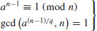

for each prime divisor q of s. Then each prime divisor p of n satisfies

(3.25)

Corollary 3.3 If , then n is prime.

The Goldwasser–Kilian test can be regarded as an elliptic curve analog of Pocklington’s theorem:

Theorem 3.16 (Goldwasser–Kilian) Let n be an integer greater than 1 and prime to 6, E an elliptic curve over , p a point on E, m and s two integers with . Suppose we have found a point p on E that satisfies , and that for each prime factor q of s, we have verified that . Then if p is a prime divisor of n, .

Corollary 3.4 If , then n is prime.

Combining the above theorem with Schoof’s algorithm [11] which computes in time , we obtain the following Goldwasser–Kilian algorithm ([5, 10]).

Algorithm 3.2 (Goldwasser–Kilian Algorithm) Given a probable prime n, this algorithm will show whether or not n is indeed prime.

1. Choose a non-singular elliptic curve E over , for which the number of points m satisfies m = 2q, with q a probable prime;

2. If (E, m) satisfies the conditions of Theorem 3.16 with s = m, then n is prime, otherwise it is composite;

3. Perform the same primality proving procedure for q;

4. Exit.

The running time of the Goldwasser–Kilian algorithm is given in the following two theorems [12]:

Theorem 3.17 Suppose that there exist two positive constants c1 and c2 such that the number of primes in the interval , where , is greater than , then the Goldwasser–Kilian algorithm proves the primality of n in expected time .

Theorem 3.18 There exist two positive constants c3 and c4 such that, for all , the proportion of prime numbers n of k bits for which the expected time of Goldwasser–Kilian is bounded by c3((log n)11) is at least

A serious problem with the Goldwasser–Kilian test is that Schoof’s algorithm seems almost impossible to implement. In order to avoid the use of Schoof’s algorithm, Atkin and Morain [12] in 1991 developed a new implementation method called ECPP (elliptic curve primality proving), which uses the properties of elliptic curves over finite fields related to complex multiplication. We summarize the principal properties of ECPP as follows:

Theorem 3.19 (Atkin–Morain) Let p be a rational prime number that splits as the product of two principal ideals in a field : with , integers of . Then there exists an elliptic curve E defined over having complex multiplication by the ring of integers of , whose cardinality is

(3.26)

with (Hasse’s theorem) and whose invariant is a root of a fixed polynomial HD(X) (depending only upon d) modulo p.

For more information on the computation of the polynomials HD, readers are referred to Cox [8] and Morain ([14, 16]). Note that there are also some other important improvements on the Goldwasser–Kilian test, notably the Adleman–Huang’s primality proving algorithm [17] using hyperelliptic curves.

The Goldwasser–Kilian algorithm begins by searching for a curve and computes its number of points, but the Atkin–Morain ECPP algorithm does exactly the opposite. The following is a brief description of the ECPP algorithm.

Algorithm 3.3 (Atkin–Morain ECPP) Given a probable prime n, this algorithm will show whether or not n is indeed prime.

1. (Initialization) Set and .

2. (Building the sequence) While Ni>Nsmall

2.1. Find a Di such that ;

2.2. If one of the w(−Di) numbers where is a conjugate of ) is probably factored go to step [2.3] else go to [2.1];

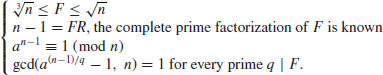
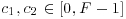
2.3. Store where mr = FiNi + 1. Here Fi is a completely factored integer and Ni + 1 a probable prime; set and go to step [2.1].

3. (Proving)

For i from k down to 0

3.1. Compute a root j of ;

3.2. Compute the equation of the curve Ei of the invariant j and whose cardinality modulo Ni is mi;

3.3. Find a point pi on the curve Ei;

3.4. Check the conditions of Theorem 3.19 with s = Ni + 1 and m = mi.

4. (Exit) Terminate the execution of the algorithm.

For ECPP, only the following heuristic analysis is known [14].

Theorem 3.20 The expected running time of the ECPP algorithm is roughly proportional to for some .

Corollary 3.5 The ECPP algorithm is in .

Thus, for all practical purposes, we could just simply use a combined test of a probabilistic test and an elliptic curve test as follows:

Algorithm 3.4 (Practical primality testing) Given a random odd positive integer n, this algorithm will make a combined use of probabilistic tests and elliptic curve tests to determine whether or not n is prime:

1. (Primality Testing – Probabilistic Testing) Use a combination of the strong pseudoprimality test and the Lucas pseudoprimality test to determine if n is a probable prime. (This has been implemented in Maple function isprime.) If it is, go to [2], else report that n is composite and go to [3].

2. (Primality Proving – Elliptic Curve Proving) Use an elliptic curve test (e.g., the ECPP test) to verify whether or not n is indeed a prime. If it is, then report that n is prime, otherwise, report that n is composite.

3. (Exit) Terminate the algorithm.

Problems for Section 3.3

1. Prove Cox’s Theorem, (i.e., Theorem 3.14) for elliptic curve primality test.

2. Prove the following theorem: Let n = FR + 1, where 0<R<F. If for some a we have

Then n is a prime.

3. (Selfridge) Let n>1 be an odd integer. Show that if

where are primes and each pi there exists an ai such that

then n is a prime.

4. Prove the Goldwasser–Kilian theorem (Theorem 3.16) and its corollary (Corollary 3.4).

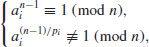
5. Show that the Goldwasser–Kilian elliptic curve test algorithm is a algorithm.

6. Show that the Atkin–Morain ECPP algorithm is a algorithm.

7. Use Cox’s test (Theorem 3.14) to prove that 26869 is a prime.

8. Use the Goldwasser–Kilian elliptic curve test to show that 907 is a prime.

9. Use some variant of ECPP to prove the following four numbers are prime:

1. ,

2. 2177580 + 5802177,

3. 44052638 + 26384405,

4. 109999 + 33603.

3.4 AKS Test

On 6 August 2002, Agrawal, Kayal, and Saxena in the Department of Computer Science and Engineering, Indian Institute of Technology, Kanpur, proposed a deterministic polynomial-time test (AKS test for short) for primality [18], relying on no unproved assumptions. That is, AKS runs in . It was not a great surprise that such a test existed,1 but the relatively easy algorithm and proof was indeed a big surprise. The key to the AKS test is in fact a very simple version of Fermat’s little theorem:

Theorem 3.21 Let x be an indeterminate and with n>1. Then

(3.27)

Proof: By the binomial theorem, we have

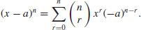
If n is prime, then (i.e., ), for . Thus, and (3.27) follows from Fermat’s little theorem. On the other hand, if n is composite, then it has a prime divisor q. Let qk be the greatest power of q that divides n. Then qk does not divide (nq) and is relatively prime to an−q, so the coefficient of the term xq on the left of 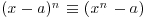is not zero, but it is on the right.

Remark 3.7 In about 1670 Leibniz (1646–1716) used the fact that if n is prime then n divides the binomial coefficient (nr), to show that if n is prime then n divides (a1 + a2 + ··· + am)n−(an1 + an2 + ··· + anm). Letting ai = 1, for , Leibniz proved that n divides mn−m for any positive integer m.

Example 3.9 Let a = 5 and n = 11. Then we have:

However, if we let n = 12, which is not a prime, then

Theorem 3.21 provides a deterministic test for primality. However, the test cannot be done in polynomial-time because of the intractability of (x−a)n; we need to evaluate n coefficients in the left-hand side of (3.27) in the worst case. A simple way to avoid this computationally intractable problem is to evaluate both sides of (3.27) modulo a polynomial2 of the form xr−1: For an appropriately chosen small r. Thus, we get a new characterization of primes

(3.28)

for all r and n relatively prime to a. A problem with this characterization is that for particular a and r, some composites can satisfy (3.28), too. However, no composite n satisfies (3.28) for all a and r, that is,

(3.29)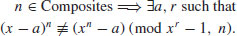

Example 3.10 Let n = 6 and a = r = 5. Then

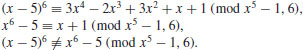
The main idea of the AKS test is to restrict the range of a and r enough to keep the complexity of the computation polynomial, while ensuring that no composite n can pass (3.28).

Theorem 3.22 (Agrawal–Kayal–Saxena) Let . Let q and r be prime numbers. Let s be a finite set of integers. Assume that

1. ,

2. ,

3. , for all distinct ,

4. ,

5. , for all .

Then n is a prime power.

Proof: We follow the streamlined presentation of Bernstein [20]. First find a prime factor p of n, with and . If every prime factor p of n has , then . By assumption, we have for all . Substituting for x, we get , and also . By induction, for all . By Fermat’s little theorem, for all . Now consider the products nipj, with and . There are such (i, j) pairs, so there are (by the pigeon-hole principle) distinct pairs (i1, j1) and (i2, j2) for which where , . So, , therefore, for all . Next find an irreducible polynomial h(x) in dividing (xr−1)/(x−1) such that for all . Define G as a subgroup of generated by , then for all . Since G has at least elements (by some combinatorics and the elementary theory of cyclotomic polynomials), we have

so, t1 = t2, as desired.

Remark 3.8 There are some new interesting developments and refinements over the above result. The American Institute of Mathematics had a workshop on 24–28 March 2003 on “Future Directions in Algorithmic Number Theory”; the institute has made the lecture notes and a set of problems of the workshop available through http://www.aimath.org.

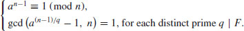
To turn the above theorem into a deterministic polynomial-time test for primality, we first find a small odd prime r such that and ; here q is the largest prime factor of r−1, and s is any moderately large integer. A theorem of Fouvry [21] from analytic number theory implies that a suitable r exists on the order and s on the order . Given such a triple (q, r, s), we can easily test that n have no prime factors <s and that for all . Any failure of the first test reveals a prime factor of n and any failure of the second test proves that n is composite. If n passes both tests then n is a prime power. Here is the algorithm.

Algorithm 3.5 (The AKS algorithm) Give a positive integer n>1, this algorithm will decide whether or not n is prime in deterministic polynomial-time.

1. If n = ab with and b>1, then output COMPOSITE.

2. Find the smallest r such that ordr(n)>4(log n)2.

3. If for some , then output COMPOSITE.

4. If , then output PRIME.

5. For a = 1 to do

if ,

then output COMPOSITE.

6. Output PRIME.

The algorithm is indeed very simple and short (with only 6 statements), possibly the shortest algorithm for a (big) unsolved problem ever!

Theorem 3.23 (Correctness) The above algorithm returns PRIME if and only if n is prime.

Proof: If n is prime, then the steps 1 and 3 will never return COMPOSITE. By Theorem 3.21, the for loop in step 5 will also never return COMPOSITE. Thus, n can only be identified to be PRIME in either step 4 or step 6. The “only if” part of the theorem left as an exercise.

Theorem 3.24 The AKS algorithm runs in time .

Proof (Sketch): The algorithm has two main steps, 2 and 5. Step 2 finds a suitable r (such an r exists by Fouvry [21] and Baker and Harman [22]), and can be carried out in time . Step 5 verifies (3.28), and can be performed in time . So, the overall runtime of the algorithm is .

Remark 3.9 Under the assumption of a conjecture on the density of the Sophie Germain primes, the AKS algorithm runs in time . If a conjecture of Bhatacharjee and Pandey3 is true, then this can be further reduced to . Of course, we do not know if these conjectures are true.

Remark 3.10 The AKS algorithm is a major breakthrough in computational number theory. However, it can only be of theoretical interest, since its current runtime is in , which is much higher than for ECPP and for Miller–Rabin’s test. For all practical purposes, we would still prefer to use Miller–Rabin’s probabilistic test [2] in the first instance and the zero-error probabilistic test ECPP in the last step of a primality testing process.

Remark 3.11 The efficiency of the AKS algorithm for test primality does not have (at least at present) any obvious connections to that of integer factorization, although the two problems are related to each other. The fastest factoring algorithm, namely the Number Field Sieve [25], has an expected running time . We do not know if the simple mathematics used in the AKS algorithm for primality testing can be used for other important mathematical problems, such as the Integer Factorization Problem.

Remark 3.12 The efficiency of the AKS algorithm has not yet become a threat to the security of the factoring base (such as the RSA) cryptographic systems, since the security of RSA depends on the computational intractability of the Integer Factorization Problem.

At the end of this section on AKS test, and also the end of this chapter on primality testing, we have given a comparison of some general purpose primality tests in terms of computational complexity (running time).

Recall that multiplying two log n bit integers has a running time of

and the fastest known algorithm, the Schönhage–Strassen algorithm, has a running time of

Thus, if we let be the running time of integer multiplication, then

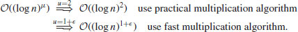
The Miller–Rabin test runs in time

so it is a very fast (polynomial-time) primality test, as its degree of complexity is just one more than integer multiplications. A drawback of the Miller–Rabin test is that it is probabilistic, not deterministic, that is, there will be a small error of probability when it declares an integer to be prime. However, if we assume the Generalized Riemann Hypothesis (GRH), then the Miller–Rabin test can be made deterministic with running time in

It still has polynomial-time complexity, just two degrees higher than its probabilistic version.

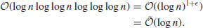
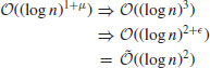
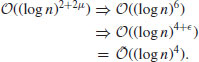
The AKS (Agrawal, Kayal, and Saxena) test takes time

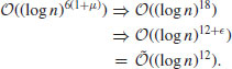
That is, by practical multiplication algorithm, AKS runs in whereas by SchönhageStrassen algorithm in . It can be show that [13] the AKS algorithm cannot be expected to be proved to run faster than

However, in practice, it is easy to find a suitable prime of the smallest possible size , thus, the practical running time of the AKS algorithm is

It also can be shown that one cannot find a deterministic test that runs faster than . That is, is the fastest possible running time for a deterministic primality test. Recently, H. Lenstra and Pomerance showed that a test having running time in

is possible, but which is essentially the same as the practical running time . Of course, if one is willing to accept a small error of probability, a randomized version of AKS is possible and can be faster, but this is not the point, as if one is willing to use a probabilistic test, one would prefer to use the Miller–Rabin test.

The APR (Adleman, Pomerance, and Rumely) cyclotomic (or Jacobi sum) test is a deterministic and nearly polynomial-time test, and it runs in time

In fact, Odlyzko and Pomerance have shown that for all large n, the running time is in the interval

where c1, c2>0. This test was further improved by Lenstra and Cohen, hence the name APRCL test. It can be used to test numbers of several thousand digits in less than, say, ten minutes.

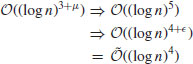
The elliptic curve test ECPP of Atkin and Morain, based on earlier work Goldwasser and Kilian, runs in time

That is, it runs in if a practical multiplication algorithm is used and if a fast multiplication algorithm is employed. ECPP is a probabilistic algorithm but with zero error; other names for this type of probabilistic algorithms are the ZPP algorithm or Las Vegas algorithm.

In what follows, Table 3.1 summarizes the running times for all the different tests mentioned in this section.

Table 3.1 Running time comparison of three general primality tests

Test	Practical running time	Fast running time
Miller–Rabin
AKS
ECPP

Brent [24] at Oxford University (now at the Australian National University) did some numerical experiments for the comparison of the Miller–Rabin, ECPP, and AKS tests on a 1GHz machine for the number 10100 + 267. Table 3.2 gives times for Magama (a computer algebra system) implementation of of the Miller–Rabin, ECPP, and AKS tests, plus our experiment on a Fujitsu P7230 Laptop computer, all for the number 10100 + 267.

Table 3.2 Times for various tests for 10100 + 267

Test	Trials	Time
Miller–Rabin	1	0.003 second
Miller–Rabin	10	0.03 second
Miller–Rabin	100	0.3 second
ECPP		2.0 seconds
Maple Test		2.751 seconds
(Miller–Rabin + Lucas)
AKS		37 weeks (Estimated)

Finally, we wish to mention that there is a practical primality test specifically for Mersenne primes numbers:

Algorithm 3.6 (Lucas–Lehmer test for Mersenne primes)

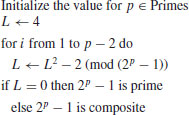
Remark 3.13 The above Lucas–Lehmer test for Mersenne primes is very efficient, since the major step in the algorithm is to compute

which can be performed in polynomial-time. But still, the computation required to test a single Mersenne prime Mp increases with p to the order of . Thus, to test M2r + 1 would take approximately eight times as long as to test Mr with the same algorithm (Slowinski [26]). Historically, it has required about four times as much computation to discover the next Mersenne prime as to re-discover all previously known Mersenne primes. The search for Mersenne primes has been an accurate measure of computing power for the past 200 years and, even in the modern era, it has been an accurate measure of computing power for new supercomputers.

Problems for Section 3.4

1. (Binomial Theorem) Prove that

where

2. Prove that

for all variables x and y and primes n.

3. Prove that n is prime if and only if

in .

4. Show that if a square root x of 1 modulo n which is neither 1 nor −1, then n is composite.

5. It is easy to find a square modulo an odd prime p, however, it is hard to find a nonsquare modulo an odd prime p. Show that, by the Extended Riemann Hypothesis, there is a nonsquare less than or equal to 2(log p)2.

6. (AKS) Let be an integer, r a positive integer <p, for which n has order greater than (log n)2 modulo r. Then n is prime if and only if

1. n is not a perfect power,

2. n does not have any prime divisor less than or equal to r,

3. for each integer a, .

7. (Bernstein) Let f(x) be a monic polynomial of degree and n positive integer. is called an almostfield with parameters (e, v(x)) if

1. , with E positive integer,

2. ,

3. is a unit in for all prime .

If n is a prime and f(x) modulo n is irreducible, then is a field. Moreover, any generator v(x) of the multiplicative group of elements of this field satisfies (2) and (3) for each E satisfying (1).

Prove that for n>2 and let be an almostfield with parameters (e, v(x)) where e>(2dlog n)2, then n is prime if and only if

a. n is not a perfect power,

b. .

8. (Lenstra, 1985) Add one more condition (4) in Problem 7:

4. .

Show that for some , and for each prime .

9. (Lenstra–Pomerance) Let f(x) be a monic polynomial of degree and n positive integer. is called a pseudofield if

1. ,

2. ,

3. is a unit in for all prime .

Prove that for and let be a pseudofield with f(x) a monic polynomial of degree d in ((log n)2, n), then n is prime if and only if

a. n is not a perfect power,

b. n does not have any prime divisor less than or equal to d,

c. , for each integer a, .

10. (AKS) Let be an integer, r a positive integer <p, for which n has order greater than (log n)2 modulo r. Then n is prime if and only if

1. n is not a perfect power,

2. n does not have any prime divisor less than or equal to r,

3. for each integer a, .

11. (Pomerance–Odlyzko) Let f(n) be the least positive square-free integer such that the product of all primes q, exceeds . Show that there exists positive absolute constants c1, c2 such that for all integers ,

12. (Adleman–Pomerance–Rumely) Let T(n) be the number of bit operations needed by the APR test. Show that there exists positive absolute constants c3, c4 such that

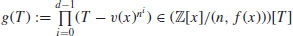
13. Prove the following theorem. Let p and q be primes with , the primitive pqth roots of unity in , g the generator of . Let also be a character of with order p. Define the Gauss sum as follows

If n is a prime, then

14. Prove that if

is true, then for any prime divisor r of n, there is a number b modulo p, such that

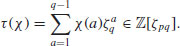
3.5 Bibliographic Notes and Further Reading

Primality testing is a large topic in computational number theory. Although primality testing problems are now proved to be solvable in polynomial-time, there is still a room for improvement to make it practically efficient. For general references on primality testing, including the historical development of efficient algorithms for primality, see, [8,13,17,19,27-49].

The original sources for the Miller–Rabin test and many other types of probabilistic primality tests (pseudoprimality tests) can be found in, for example, [1–3, 24, 50–56].

The elliptic curve primality test was first proposed by Goldwasser and Kilian in [5, 10, 57], but the most practical and fastest version of elliptic curve primality test, ECPP, was proposed and improved in [12, 14–16]. Gross [58] discussed the application of elliptic curve test for Mersenne primes.

The AKS deterministic polynomial-time primality test was proposed by Agrawal, Kayal, and N. Saxena in [18]. More discussions and improvements of AKS test may be found in [20, 23, 59,60]. Prior to AKS, the super-polynomial-time primality test APR was proposed by Adleman, Pomerance, and Rumely in 1983 [61], and subsequently improved by Cohen and Lenstra in 1984 [62].

References

1. G. Miller, “Riemann’s Hypothesis and Tests for Primality”, Journal of Systems and Computer Science, 13, 1976, pp. 300–317.

2. M. O. Rabin, “Probabilistic Algorithms for Testing Primality”, Journal of Number Theory, 12, 1980, pp. 128–138.

3. V. R. Pratt, “Every Prime Has a Succinct Certificate”, SIAM Journal on Computing, 4, 1975, pp. 214–220.

4. H. W. Lenstra, Jr., “Factoring Integers with Elliptic Curves”, Annals of Mathematics, 126, 1987, pp. 649–673.

5. S. Goldwasser and J. Kilian, “Almost All Primes Can be Quickly Certified”, Proceedings of the 18th ACM Symposium on Theory of Computing, Berkeley, 1986, pp. 316–329.

6. V. Miller, “Uses of Elliptic Curves in Cryptography”, Lecture Notes in Computer Science, 218, Springer, 1986, pp. 417–426.

7. N. Koblitz, “Elliptic Curve Cryptography”, Mathematics of Computation, 48 1987, pp. 203–209.

8. D. A. Cox, Primes of the Form x2 + ny2, Wiley, 1989.

9. R. A. Mollin, Introduction to Cryptography, 2nd Edition, CRC Press, 2006.

10. S. Goldwasser and J. Kilian, “Primality Testing Using Elliptic Curves”, Journal of ACM, 46, 4, 1999, pp. 450–472.

11. R. Schoof, “Elliptic Curves over Finite Fields and the Computation of Square Roots ”, Mathematics of Computation, 44, 1985, pp. 483–494.

12. A. O. L. Atkin and F. Morain, “Elliptic Curves and Primality Proving”, Mathematics of Computation, 61, 1993, pp. 29–68.

13. R. Schoof, “Four Primality Testing Algorithms”, Algorithmic Number Theory. Edited by J. P. Buhler and P. Stevenhagen, Cambridge University Press, 2008, pp. 69–81.

14. F. Morain, Courbes Elliptiques et Tests de Primalité, Université Claude Bernard, Lyon I, 1990.

15. F. Morain, “Primality Proving Using Elliptic Curves: An Update”, Algorithmic Number Theory, Lecture Notes in Computer Science 1423, Springer, 1998, pp. 111–127.

16. F. Morain, “Implementing the Asymptotically Fast Version of the Elliptic Curve Primality Proving Algorithm”, Mathematics of Computation, 76, 2007, pp. 493–505.

17. L. M. Adleman and M. D. A. Huang, Primality Testing and Abelian Varieties over Finite Fields, Lecture Notes in Mathematics 1512, Springer-Verlag, 1992.

18. M. Agrawal, N. Kayal, and N. Saxena, “Primes is in P”, Annals of Mathematics, 160, 2, 2004, pp. 781–793.

19. J. D. Dixon, “Factorization and Primality tests”, The American Mathematical Monthly, June–July 1984, pp. 333–352.

20. D. J. Bernstein, Proving Primality After Agrawal-Kayal-Saxena, Dept of Mathematics, Statistics and Computer Science, The University of Illinois at Chicago, 25 Jan 2003.

21. E. Fouvry, “Theorème de Brun-Titchmarsh: Application au Theorème de Fermat”, ventiones Mathematicae, 79, 1985, pp. 383–407.

22. R. C. Baker and G. Harman, “The Brun-Tichmarsh Theorem on Average”, in Proceedings of a Conference in Honor of Heini Halberstam, Volume 1, 1996, pp. 39–103.

23. R. Bhattacharjee and P. Pandey, Primality Testing, Dept of Computer Science & Engineering, Indian Institute of Technology Kanpur, India, 2001.

24. R. P. Brent, “Uncertainty Can Be Better Than certainty: Some Algorithms for Primality Testing”, Mathematical Institute, Australian National University, 2006.

25. A. K. Lenstra and H. W. Lenstra, Jr. (eds), The Development of the Number Field Sieve, Lecture Notes in Mathematics 1554, Springer-Verlag, 1993.

26. D. Slowinski, “Searching for the 27th Mersenne Prime”, Journal of Recreational Mathematics, 11, 4, 1978–79, pp. 258–261.

27. L. M. Adleman, “Algorithmic Number Theory – The Complexity Contribution”, Proceedings of the 35th Annual IEEE Symposium on Foundations of Computer Science, IEEE Press, 1994, pp. 88–113.

28. E. Bach and J. Shallit, Algorithmic Number Theory I – Efficient Algorithms, MIT Press, 1996.

29. R. P. Brent, “Primality Testing and Integer Factorization”, in Proceedings of Australian Academy of Science Annual General Meeting Symposium on the Role of Mathematics in Science, Canberra, 1991, pp. 14–26.

30. D. M. Bressound, Factorization and Primality Testing, Springer, 1989.

31. H. Cohen, A Course in Computational Algebraic Number Theory, Graduate Texts in Mathematics 138, Springer-Verlag, 1993.

32. T. H. Cormen, C. E. Ceiserson, and R. L. Rivest, Introduction to Algorithms, 3rd Edition, MIT Press, 2009.

33. R. Crandall and C. Pomerance, Prime Numbers – A Computational Perspective, 2nd Edition, Springer-Verlag, 2005.

34. J. H. Davenport, Primality Testing Revisited, School of Mathematical Sciences, University of Bath, UK, 1992.

35. C. F. Gauss, Disquisitiones Arithmeticae, G. Fleischer, Leipzig, 1801. English translation by A. A. Clarke, Yale University Press, 1966. Revised English translation by W. C. Waterhouse, Springer-Verlag, 1975.

36. D. E. Knuth, The Art of Computer Programming II – Seminumerical Algorithms, 3rd Edition, Addison-Wesley, 1998.

37. N. Koblitz, A Course in Number Theory and Cryptography, 2nd Edition, Graduate Texts in Mathematics 114, Springer-Verlag, 1994.

38. E. Kranakis, Primality and Cryptography, Wiley, 1986.

39. H. W. Lenstra, Jr., Primality Testing Algorithms, Séminaire N. Bourbaki 1980–1981, Number 561, pp. 243–257. Lecture Notes in Mathematics 901, Springer, 1981.

40. J. M. Pollard, “Theorems on Factorization and Primality Testing”, Proceedings of Cambridge Philosophy Society, 76, 1974, pp. 521–528.

41. C. Pomerance, “Very Short Primality Proofs”, Mathematics of Computation, 48, 1987, pp. 315–322.

42. C. Pomerance, “ Computational Number Theory”, In: Princeton Companion to Mathematics, W. T. Gowers, (ed.) Princeton University Press, 2008, pp. 348–362.

43. H. Riesel, Prime Numbers and Computer Methods for Factorization, Birkhäuser, Boston, 1990.

44. K. Rosen, Elementary Number Theory and its Applications, 5th Edition, Addison-Wesley, 2005.

45. R. Rumely, “Recent Advances in Primality Testing”, Notices of the AMS, 30, 8, 1983, pp. 475–477.

46. V. Shoup, A Computational Introduction to Number Theory and Algebra, Cambridge University Press, 2005.

47. S. Wagon, “Primality Testing”, The Mathematical Intelligencer, 8, 3, 1986, pp. 58–61.

48. H. S. Wilf, Algorithms and Complexity, 2nd Edition, A. K. Peters, 2002.

49. S. Y. Yan, Primality Testing and Integer Factorization in Public-Key Cryptography, Advances in Information Security 11, 2nd Edition, Springer, 2009.

50. W. Alford, G. Granville, and C. Pomerance, “There Are Infinitely Many Carmichael Numbers”, Annals of Mathematics, 140, 1994, pp. 703–722.

51. A. Granville, “Primality Testing and Carmichael Numbers”, Notice of the American Mathematical Society, Vol 39, 1992, pp. 696–700.

52. C. Pomerance, “Primality Testing: Variations on a Theme of Lucas”, in Proceedings of the 13th Meeting of the Fibonacci Association, Congressus Numerantium, 201, 2010, pp. 301–312.

53. C. Pomerance, J. L. Selfridge and S. S. Wagstaff, Jr., “The Pseudoprimes to ”, Mathematics of Computation, 35, 1980, pp. 1003–1026.

54. P. Ribenboim, “Selling Primes”, Mathematics Magazine, 68, 3, 1995, pp. 175–182.

55. R. Solovay and V. Strassen, “A Fast Monte-Carlo Test for Primality”, SIAM Journal on Computing, 6, 1, 1977, pp. 84–85. “Erratum: A Fast Monte-Carlo Test for Primality”, SIAM Journal on Computing, 7, 1, 1978, p. 118.

56. H. C. Williams, Édouard Lucas and Primality Testing, John Wiley & Sons, 1998.

57. J. Kilian, Uses of Randomness in Algorithms and Protocols, MIT Press, 1990.

58. B. H. Gross, “An Elliptic Curve Test for Mersenne Primes”, Journal of Number Theory, 110, 2005, pp. 114–119.

59. A. Granville, “It is Easy to Determine Whether a Given Integer is Prime”, Bulletin (New Series) of the American Mathematical Society, Vol 42, 1, 2004, pp. 3–38.

60. H. W. Lenstra, Jr., and C. Pomerance, “Primality Testing with Gaussian Periods”, Department of Mathematics, Dartmouth College, Hanover, NH 03874, USA, 12 April 2011.

61. L. M. Adleman, C. Pomerance, and R. S. Rumely, “On Distinguishing Prime Numbers from Composite Numbers”, Annals of Mathematics, 117, 1, 1983, pp. 173–206.

62. H. Cohen and H. W. Lenstra, Jr., “Primality Testing and Jacobi Sums, Mathematics of Computation, 42, 165, 1984, pp. 297–330.

1Dixon [19] predicated in 1984 that “the prospect for a polynomial-time algorithm for proving primality seems fairly good, but it may turn out that, on the contrary, factoring is NP-hard.”

2By analog with congruences in , we say that polynomials f(x) and g(x) are congruent modulo h(x) and write , whenever f(x)−g(x) is divisible by h(x). The set (ring) of polynomials modulo h(x) is denoted by . If all the coefficients in the polynomials are also reduced to n, then we write as , and as (or if n is a prime p).

3 Bhatacharjee and Pandey conjectured in 2001 [23] that if and , and , then either n is prime or .