4

Integer Factorization

The Integer Factorization Problem (IFP) is one of the most important infeasible problems in computational number theory, for which there is still no polynomial-time algorithm for solving it. In this chapter we discuss several important modern algorithms for factoring, including

• Pollard’s and p−1 Methods;
• Lenstra’s Elliptic Curve Method (ECM);
• Pomerance’s Quadratic Sieve (QS), and
• The currently fastest method, Number Field Sieve (NFS).

4.1 Basic Concepts

The Integer Factorization Problem (IFP) may be described as follows:

(4.1)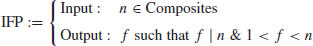

Clearly, if there is an algorithm to test whether or not an integer n is a prime, and an algorithm to find a nontrivial factor f of a composite integer n, then by recursively calling the primality testing algorithm and the integer factorization algorithm, it should be easy to find the prime factorization of

Generally speaking, the most useful factoring algorithms fall into one of the following two main classes:

A. General purpose factoring algorithms, which has running time that depends mainly on the size of n, the number to be factored, and is not strongly dependent on the size of the factor p found. Examples are:

1. Lehman’s method, which has a rigorous worst-case running time bound .

2. Shanks’ SQUare FOrm Factorization methodSQUFOF, which has expected running time .

3. Shanks’ class group method, which has running time .

4. Continued FRACtion (CFRAC) method, which under plausible assumptions has expected running time

where c is a constant (depending on the details of the algorithm); usually .

5. Multiple Polynomial Quadratic Sieve (MPQS), which under plausible assumptions has expected running time

where c is a constant (depending on the details of the algorithm); usually .

6. Number Field Sieve (NFS), which under plausible assumptions has the expected running time

where if GNFS (a general version of NFS) is used to factor an arbitrary integer n, whereas if SNFS (a special version of NFS) is used to factor a special integer n such as , where r and s are small, r>1 and e is large. This is substantially and asymptotically faster than any other currently known factoring method.

B. Special purpose factoring algorithms: The running time depends mainly on the size of p (the factor found) of n. (We can assume that .) Examples are:

1. Trial division, which has running time .

2. Pollard’s Method (also known as Pollard’s “rho” algorithm), which under plausible assumptions has expected running time .

3. Lenstra’s Elliptic Curve Method (ECM), which under plausible assumptions has expected running time

where is a constant (depending on the details of the algorithm).

The term is for the cost of performing arithmetic operations on numbers which are or bits long; the second can be theoretically replaced by for any .

Note that there is a quantum factoring algorithm, first proposed by Shor, which can run in polynomial-time

However, this quantum algorithm requires running on a practical quantum computer with several thousand quantum bits, which is not available at present.

In practice, algorithms in both categories are important. It is sometimes very difficult to say whether one method is better than another, but it is generally worth attempting to find small factors with algorithms in the second class before using the algorithms in the first class. That is, we could first try the trial division algorithm, then use some other method such as NFS. This fact shows that the trial division method is still useful for integer factorization, even though it is simple. In this chapter we shall introduce some most the useful and widely used factoring algorithms.

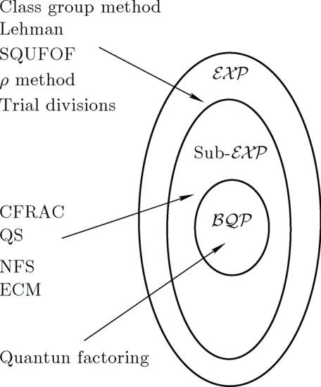
From a computational complexity point of view, the IFP is an infeasible (intractable) problem, since there is no polynomial-time algorithm for solving it; all the existing algorithms for IFP run in subexponential-time or above (see Figure 4.1).

Figure 4.1 Algorithms/Methods for IFP

Problems for Section 4.1

1. (Sierpinski) Prove that there are infinitely many integers k such that

are all composite. Find three such composites.

2. Show that the sequence contains infinitely many composites.

3. Suppose n = pq with p, q prime and p<q<2p. Let be the number defined by such that . Show that the number of steps used in the Fermat factoring method is approximately .

4. Let n = pq = 18886013 such that

Find the factorization of n.

5. Explain why general purpose factoring algorithms are slower than special purpose factoring algorithms, or why the special numbers are easy to factor than general numbers.

6. Show that addition of two log n bit integers can be performed in bit operations.

7. Show that multiplication of two log n bit integers can be performed in bit operations.

8. Show that there is an algorithm which can multiply two log n bit integers in

bit operations.

9. Show that if , then .

10. Prove or disprove that -complete.

4.2 Trial Divisions Factoring

The simplest factoring algorithm is perhaps the trial division method, which tries all the possible divisors of n to obtain its complete prime factorization:

(4.2)

The following is the algorithm:

Algorithm 4.1 (Factoring by trial divisions) This algorithm tries to factor an integer n>1 using trial divisions by all the possible divisors of n.

1. [Initialization] Input n and set , .

2. [n = 1?] If n = 1, then go to [5].

3. [Compute Remainder]

4. [Factor Found?]

5. [Exit] Terminate the algorithm.

Exercise 4.1 Use Algorithm 4.1 to factor n = 2759.

An immediate improvement of Algorithm 4.1 is to make use of an auxiliary sequence of trial divisors:

(4.3)

which includes all primes (possibly some composites as well if it is convenient to do so) and at least one value . The algorithm can be described as follows:

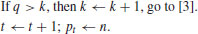
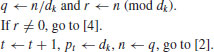
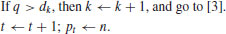
Algorithm 4.2 (Factoring by Trial Division) This algorithm tries to factor an integer n>1 using trial divisions by an auxiliary sequence of trial divisors.

1. [Initialization] Input n and set , .

2. [n = 1?] If n = 1, then go to [5].

3. [Compute Remainder]

4. [Factor Found?]

5. Exit: terminate the algorithm.

Exercise 4.2 Use Algorithm 4.2 to factor n = 2759; assume that we have the list L of all primes 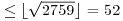and at least one , that is, .

Theorem 4.1 Algorithm 4.2 requires a running time in

If a primality test between steps [2] and [3] were inserted, the running time would then be in , or if one does trial division only by primes, where pt−1 is the second largest prime factor of n.

The trial division test is very useful for removing small factors, but it should not be used for factoring completely, except when n is very small, say, for example, n<108.

Algorithm 4.2 seems to be very simple, but its analysis is rather complicated. For example, in order to analyse the average behavior of the algorithm, we will need to know how many trial divisions are necessary and how large the largest prime factor pt will tend to be.

Let be the primes . Then, if the Riemann Hypothesis is true, it would imply that

(4.4)

where . In 1930, Karl Dickman investigated the probability that a random integer between 1 and x will have its largest prime factor . He gave a heuristic argument to show that this probability approaches the limiting value as , where f can be calculated from the functional equation

(4.5)

His argument was essentially this: Given 0<t<1, the number of integers less than x whose largest prime factor is between xt and xt + dt is . The number of prime p in that range is

(4.6)

For every such p, the number of integers n such that “ and the largest prime factor of n is ” is the number of whose largest prime factor is , namely x1−tF(t/(1−t)). Hence and (4.5) follows by integration.

If , formula (4.5) simplifies to

(4.7)

Thus, for example, the probability that a random positive integer has a prime factor is , In all such cases, Algorithm 4.2 must work hard. So, practically, Algorithm 4.2 will give the answer rather quickly if we want to factor a 6-digit integer; but for large n, the amount of computer time for factoring by trial division will rapidly exceed practical limits, unless we are unusually lucky. The algorithm usually finds a few small factors and then begins a long-drawn-out search for the large ones that are left. Interested readers are referred to [4] for more detailed discussion.

By an argument analogous to Dickman’s, it has been shown that the second largest prime factor of a random integer x will be with approximate probability , where

(4.8)

Clearly, for .

The total number of prime factors, t is obviously , but these lower and upper bounds are seldom achieved. It is possible to prove that if n is chosen at random between 1 and x, the probability that approaches

(4.9)

as , for any fixed c. In other words, the distribution of t is essentially normal, with mean and variance ln ln x; about 99.73 % of all the large integers have . Furthermore, the average value of t−ln ln x for is known to approach

(4.10)

It follows from the above analysis that Algorithm 4.2 will be useful for factoring a 6-digit integer, or a large integer with small prime factors. Fortunately, many more efficient factorization algorithms have been developed since 1980, requiring fewer bit operations than the trial division method; with the fastest being the Number Field Sieve (NFS), which will be discussed later.

Problems for Subsection 4.2

1. (Hardy and Littlewood, 1918) Show that there is a positive real constant c such that

for infinitely many x.

2. Let pt be the largest prime factor of a random integer n between 1 and x. What is the probability that n has its largest prime factor ?

3. Let pt−1 be the second largest prime factor of a random integer n between 1 and x. What is the probability that n has its second largest prime factor ?

4. Let t be the total number of prime factors of n between 1 and x. What is the probability that for any fixed c, as ?

5. Suppose n = pq with p, q prime and p<q<2p. Let be the number defined by such that . Show that the number of steps used in the Fermat factoring method is approximately .

6. Let p be an od prime and for . Show that the number of solutions of (x, y) to with is equal to .

7. Let n be an odd integer. Show that if n can be factored as

then n can be written as a difference of the two squares x2 and y2, where

8. The Fermat factoring method is based on the fact that if n is a difference of the two squares such as x2 and y2, then n can be factored as n = (x−y)(x + y). Use the Fermat factoring method to factor the numbers 1254713 and 2027651281.

9. Show that the Fermat factoring method is of the complexity .

4.3 ρ and p−1 Methods

In 1975 John M. Pollard proposed a very efficient Monte Carlo method [2], now widely known as Pollard’s “rho” or Method, for finding a small nontrivial factor d of a large integer n. Trial division by all integers up to is guaranteed to factor completely any number up to n. For the same amount of work, Pollard’s “rho” Method will factor any number up to n2 (unless we are unlucky).

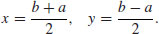
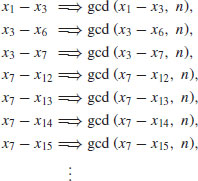
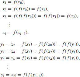
The method uses an iteration of the form

(4.11)

where x0 is a random starting value, n is the number to be factored, and is a polynomial with integer coefficients; usually, we just simply choose with . Then starting with some initial value x0, a “random” sequence is computed modulo n in the following way:

(4.12)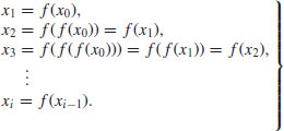

Let d be a nontrivial divisor of n, where d is small compared with n. Since there are relatively few congruence classes modulo d (namely, d of them), there will probably exist integers xi and xj which lie in the same congruence class modulo d, but belong to different classes modulo n; in short, we will have

(4.13)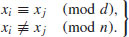

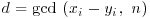
Since and , it follows that is a nontrivial factor of n. In practice, a divisor d of n is not known in advance, but it can most likely be detected by keeping track of the integers xi, which we do know; we simply compare xi with the earlier xj, calculating 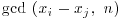until a nontrivial gcd occurs. The divisor obtained in this way is not necessarily the smallest factor of n and indeed it may not be prime. The possibility exists that when a gcd greater that 1 is found, it may also turn out to be equal to n itself, though this happens very rarely.

Example 4.1 For example, let , f(x) = x2−1 and x1 = 2. Then the “random” sequence is as follows:

where the repeated values are overlined. Now we find that

So we have

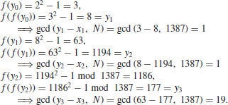
Of course, as mentioned earlier, d is not known in advance, but we can keep track of the integers xi which we do know, and simply compare xi with all the previous xj with j<i, calculating 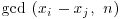until a nontrivial gcd occurs:

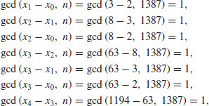
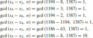
So after 13 comparisons and calculations, we eventually find the divisor 19.

As k increases, the task of computing for all j<i becomes very time-consuming; for n = 1050, the computation of would require about bit operations, as the complexity for computing one gcd is . Pollard actually used Floyd’s method to detect a cycle in a long sequence , which just looks at cases in which xi = x2i. To see how it works, suppose that , then

(4.14)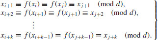

If k = j−i, then 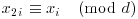. Hence, we only need look at x2i−xi (or xi−x2i) for . That is, we only need to check one gcd for each i. Note that the sequence modulo a prime number p, say, looks like a circle with a tail; it is from this behavior that the method gets its name (see Figure 4.2 for a graphical sketch; it looks like the Greek letter ).

Figure 4.2 Illustration of the Method

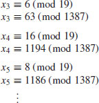
Example 4.2 Again, let , f(x) = x2−1, and x1 = 2. By comparing pairs xi and x2i, for , we have:

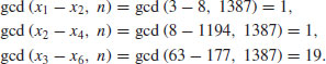
So after only three comparisons and gcd calculations, the divisor 19 of 1387 is found.

In what follows, we shall show that to compute yi = x2i, we do not need to compute 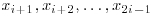until we get x2i. Observe that

(4.15)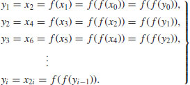

So at each step, we compute

(4.16)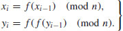

Therefore, only three evaluations of f will be required.

Example 4.3 Let once again 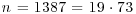, f(x) = x2−1, and x0 = y0 = 2. By comparing pairs xi and x2i, for , we get:

The divisor 19 of 1387 is then found.

Remark 4.1 There is an even more efficient algorithm, due to Richard Brent [3], that looks only at the following differences and the corresponding gcd results:

and in general:

(4.17)

Brent’s algorithm is about 24% faster than Pollard’s original version.

Now we are in a position to present an algorithm for the Method.

Algorithm 4.3 (Brent–Pollard’s Method) Let n be a composite integer greater than 1. This algorithm tries to find a nontrivial factor d of n, which is small compared to . Suppose the polynomial to use is f(x) = x2 + 1.

1. (Initialization) Choose a seed, say x0 = 2, a generating function, say . Choose also a value for t not much bigger than , perhaps .

2. (Iteration and Computation) Compute xi and yi in the following way:

and simultaneously compare xi and yi by computing .

3. (Factor Found?) If 1<d<n, then d is a nontrivial factor of n, print d, and go to Step [5].

4. (Another Search?) If for some i or , then go to Step [1] to choose a new seed and a new generator and repeat.

5. (Exit) Terminate the algorithm.

Example 4.4 The 8th Fermat number was factored by Brent and Pollard in 1980 by using Brent–Pollard’s “rho” Method:

Now let us move to consider the complexity of the Method. Let p be the smallest prime factor of n, and j the smallest positive index such that . Making some plausible assumptions, it is easy to show that the expected value of j is . The argument is related to the well-known “birthday” paradox: Suppose that and that the numbers are independently chosen from the set . Then the probability that the numbers xk are distinct is

(4.18)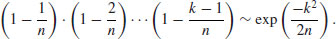

Note that the xi’s are likely to be distinct if k is small compared with , but unlikely to be distinct if k is large compared with . Of course, we cannot work out , since we do not know p in advance, but we can detect xj by taking greatest common divisors. We simply compute for and stop when a d>1 is found.

Conjecture 4.1 (Complexity of the Method) Let p be a prime dividing n and , then the algorithm has expected running time

(4.19)

to find the prime factor p of n.

Remark 4.2 The Method is an improvement over trial division, because in trial division, divisions are needed to find a small factor p of n. But of course, one disadvantage of the algorithm is that its running time is only a conjectured expected value, not a rigorous bound.

In 1974, Pollard [40] also invented another simple but effective factoring algorithm, now widely known as Pollard’s “p−1” Method, which can be described as follows:

Algorithm 4.4 (Pollard’s “p−1” Method) Let n>1 be a composite number. This algorithm attempts to find a nontrivial factor of n.

1. (Initialization) Pick out at random. Select a positive integer k that is divisible by many prime powers, for example, for a suitable bound B (the larger B is the more likely the method will be to succeed in producing a factor, but the longer the method will take to work).

2. (Exponentiation) Compute .

3. (Compute GCD) Computing .

4. (Factor Found?) If 1<d<n, then d is a nontrivial factor of n, output d and go to Step [6].

5. (Start Over?) If d is not a nontrivial factor of n and if you still want to try more experiments, then go to Step [1] to start all over again with a new choice of a and/or a new choice of k, else go to Step [6].

6. (Exit) Terminate the algorithm.

The “p−1” algorithm is usually successful in the fortunate case where n has a prime divisor p for which p−1 has no large prime factors. Suppose that and that . Since , we have , thus . In many cases, we have , so the method finds a nontrivial factor of n.

Example 4.5 Use the “p−1” Method to factor the number n = 540143. Choose B = 8 and hence k = 840. Choose also a = 2. Then we have

Thus 421 is a (prime) factor of 540143. In fact, is the complete prime factorization of 540143. It is interesting to note that by using the “p−1” method Baillie in 1980 found the prime factor

of the Mersenne number M257 = 2257−1. In this case

In the worst case, where (p−1)/2 is prime, the “p−1” algorithm is no better than trial division. Since the group has fixed order p−1 there is nothing to be done except try a different algorithm. Note that there is a similar method to “p−1,” called “p + 1,” that was proposed by H. C. Williams in 1982. It is suitable for the case where n has a prime factor p for which p + 1 has no large prime factors.

Problems for Section 4.3

1. Let f be a random function in a set of p elements, and x0 a random element. Define iteratively that xi + 1 = f(xi), , for a given real number . Show that the probability are pairwise different .

2. Show that the complexity of the Method for factoring a general number n is .

3. Let n = 3161 and x0 is the seed with f(x) = x2 + 1. Use the Method to factor n.

4. Use p−1 method to find the smallest prime factor of the 9th Fermat number .

5. Use p−1 method to find three prime factors of 271−1.

6. Use the Factoring Method to factor 4087 using x0 = 2 and f(x) = x2−1.

7. Let . Let also t, u>0 be the smallest numbers in the sequence , where t and u are called the lengths of the tail and cycle, respectively. Give an efficient algorithm to determine t and u exactly, and analyze the running time of your algorithm.

4.4 Elliptic Curve Method

In this section, we shall introduce a factoring method depending on the use of elliptic curves. The method is actually obtained from Pollard’s “p−1” algorithm: If we can choose a random group G with order G close to p, we may be able to perform a computation similar to that involved in Pollard’s “p−1” algorithm, working in G rather than in Fp. If all prime factors of G are less than the bound B then we find a factor of n. Otherwise, we repeat this procedure with a different group G (and hence, usually, a different G) until a factor is found. This is the motivation of the ECM method, invented by H. W. Lenstra in 1987 [42].

Algorithm 4.5 (Lenstra’s Elliptic Curve Method) Let n>1 be a composite number, with . This algorithm attempts to find a nontrivial factor of n. The method depends on the use of elliptic curves and is the analog to Pollard’s “p−1” Method.

1. (Choose an Elliptic Curve) Choose a random pair (E, P), where e is an elliptic curve y2 = x3 + ax + b over , and is a point on e. That is, choose at random, and set . If , then e is not an elliptic curve, start all over and choose another pair (E, P).

2. (Choose an Integer k) Just as in the “p−1” Method, select a positive integer k that is divisible by many prime powers, for example, or k = B! for a suitable bound B; the larger B is the more likely the method will succeed in producing a factor, but the longer the method will take to work.

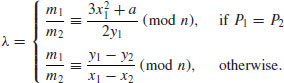
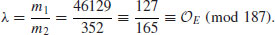
3. (Calculate kP) Calculate the point . We use the following formula to compute P3(x3, y3) = P1(x1, y1) + P2(x2, y2) modulo n:

where

The computation of can be done in doublings and additions.

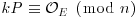4. (Computing GCD) If , then compute , else go to Step [1] to make a new choice for “a” or even for a new pair (E, P).

5. (Factor Found?) If 1<d<n, then d is a nontrivial factor of n, output d and go to Step [7].

6. (Start Over?) If d is not a nontrivial factor of n and if you still wish to try more elliptic curves, then go to Step [1] to start all over again, else go to Step [7].

7. (Exit) Terminate the algorithm.

As for the “p−1” method, one can show that a given pair (E, P) is likely to be successful in the above algorithm if n has a prime factor p for which is composed of small primes only. The probability for this to happen increases with the number of pairs (E, P) that one tries.

Example 4.6 Use the ECM method to factor the number n = 187.

1. Choose B = 3, and hence k = l cm(1, 2, 3) = 6. Let P = (0, 5) be a point on the elliptic curve E : y2 = x3 + x + 25 which satisfies (note that here a = 1 and b = 25).

2. Since k = 6 = 1102, we compute 6P = 2(P + 2P) in the following way:

a. Compute 2P = P + P = (0, 5) + (0, 5):

So 2P = (144, 18) with m2 = 10 and .

b. Compute 3P = P + 2P = (0, 5) + (144, 18):

So 3P = (124, 176) with m2 = 144 and .

c. Compute 6P = 2(3P) = 3P + 3P = (124, 176) + (124, 176):

This time m1 = 127 and m2 = 165, so the modular inverse for 127/165 modulo 187 does not exist; but this is exactly what we want! – this type of failure is called a “pretend failure.”

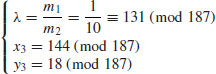
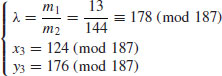
3. Compute . Since 1<11<187, 11 is a (prime) factor of 187. In fact, .

Example 4.7 To factor n = 7560636089, we calculate kP = k(1, 3) with on :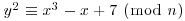

3P = (1329185554, 395213649)	6P = (646076693, 5714212282)
12P = (5471830359, 5103472059)	24P = (04270711, 3729197625)
49P = (326178740, 3033431040)	99P = (5140727517, 2482333384)
199P = (1075608203, 3158750830)	398P = (4900089049, 2668152272)
797P = (243200145, 2284975169)	1595P = (3858922333, 4843162438)
3191P = (7550557590, 1472275078)	6382P = (4680335599, 1331171175)
12765P = (6687327444, 7233749859)	25530P = (6652513841, 6306817073)
51061P = (6578825631, 5517394034)	102123P = (1383310127, 2036899446)
204247P = (3138092894, 2918615751)	408495P = (6052513220, 1280964400)
816990P = (2660742654, 3418862519)	1633980P = (7023086430, 1556397347)
3267961P = (5398595429, 795490222)	6535923P = (4999132, 4591063762)
13071847P = (3972919246, 7322445069)	26143695P = (3597132904, 3966259569)
52287391P = (2477960886, 862860073)	104574782P = (658268732, 3654016834)
209149565P = (6484065460, 287965264)	418299131P = (1622459893, 4833264668)
836598262P = (7162984288, 487850179)	.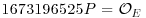

Now, 1673196525P is the point at infinity since is impossible. Hence, gives a factor of n.

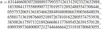
Example 4.8 The following are some ECM factoring examples. In 1995 Richard Brent at the Australian National University completed the factorization of the 10th Fermat number using ECM:

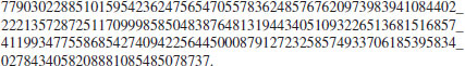
where the 40-digit prime p40 was found using ECM, and p252 was proved to be a 252-digit prime. Brent also completed the factorization of the 11th Fermat number (with 617-digit) 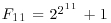using ECM:

where the 21-digit and 22-digit prime factors were found using ECM, and p564 is a 564-digit prime. Other recent ECM-records include a 38-digit prime factor (found by A. K. Lenstra and M. S. Manasse) in the 112-digit composite , a 40-digit prime factor of 26126 + 1, a 43-digit prime factor of the partition number p(19997), and a 44-digit prime factor of the partition number p(19069) in the RSA Factoring Challenge List, and a 47-digit prime in c135 of .

Both Lenstra’s ECM algorithm and Pollard’s “p−1” algorithm can be sped up by the addition of a second phase. The idea of the second phase in ECM is to find a factor in the case that the first phase terminates with a group element , such that is reasonably small, say ), here is the cyclic group generated by p. There are several possible implementations of the second phase. One of the simplest uses a pseudorandom walk in . By the birthday paradox argument, there is a good chance that two points in the random walk will coincide after steps, and when this occurs a nontrivial factor of n can usually be found (see [6] and [5] for more detailed information on the implementation issues of the ECM.

Conjecture 4.2 (Complexity of the ECM method) Let p be the smallest prime dividing n. Then the ECM method will find p of n, under some plausible assumptions, in expected running time

(4.20)

In the worst case, when n is the product of two prime factors of the same order of magnitude, we have

(4.21)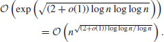

Remark 4.3 The most interesting feature of ECM is that its running time depends very much on p (the factor found) of n, rather than n itself. So one advantage of the ECM is that one may use it, in a manner similar to trial divisions, to locate the smaller prime factors p of a number n which is much too large to factor completely.

Problems for Section 4.4

1. Show that #(a, b) = p2−p, where #(a, b) denotes the number of integer pairs (a, b) such that , for which is exactly p2−p.

2. Show that if , then the root r of the congruence is a repeated rood modulo p of the polynomial x3−ax−b.

3. Let p>2 be prime. Suppose that x and y are integers such that

Let u be determined by the congruence

Show that

4. Canfield–Erdös–Pomerance theorem: Let n be a positive integer which is not a prime power and not divisible by 2 or 3. if is a real number, then the probability that a random positive integer has all its prime factors is for , where with x a real number >e.

We also need the following conjecture: Let x = p, the probability that a random integer has all its prime factors in the small interval is for .

By the Canfield–Erdös–Pomerance theorem and the conjecture, show that

1. the probabilistic time estimate for ECM to find the smallest prime factor p of n is

2. the probabilistic time estimate for ECM to find n is

5. Use Algorithm 4.5 to factor the three integers 17531, 218548425731 and 190387615311371.

6. Modify and improve Algorithm 4.5 to a practical factoring algorithm for large integer n.

7. Modify and improve Algorithm 4.5 to a parallel practical factoring algorithm for large integer n.

4.5 Continued Fraction Method

The Continued Fraction Method is perhaps the first modern, general  purpose integer factorization method, although its original idea may go back to M. Kraitchik in the 1920s, or even earlier to A. M. Legendre. It was used by D. H. Lehmer and R. E. Powers to devise a new technique in the 1930s, however the method was not very useful and applicable at the time because it was unsuitable for desk calculators. About 40 years later, it was first implemented on a computer by M. A. Morrison and J. Brillhart [7], who used it to successfully factor the seventh Fermat number

on the morning of 13 September 1970.

The Continued FRACtion (CFRAC) method looks for small values of |W| such that has a solution. Since W is small (specifically ), it has a reasonably good chance of being a product of primes in our factor base FB. Now if W is small and , then we can write x2 = W + knd2 for some k and d, hence (x/d)2−kn = W/d2 will be small. In other words, the rational number x/d is an approximation of . This suggests looking at the continued fraction expansion of , since continued fraction expansions of real numbers give good rational approximations. This is exactly the idea behind the CFRAC method! We first obtain a sequence of approximations (i.e., convergents) Pi/Qi to for a number of values of k, such that

(4.22)

Putting Wi = P2i−Q2ikn, then we have

(4.23)

Hence, the are small and more likely to be smooth, as desired. Then, we try to factor the corresponding integers Wi = P2i−Q2ikn over our factor base FB; with each success, we obtain a new congruence of the form

(4.24)

Once we have obtained at least m + 2 such congruences, by Gaussian elimination over we have obtained a congruence . That is, if (x1, e01, e11, ···, em1), ···, (xr, e0r, e1r, ···, emr) are solutions of (4.24) such that the vector sum

(4.25)

is even in each component, then

(4.26)

(4.27)

is a solution to

(4.28)

except for the possibility that , and hence (usually) a nontrivial factoring of n, by computing .

Example 4.9 We now illustrate, by an example, the idea of CFRAC factoring. Let n = 1037. Then . The first ten continued fraction approximations of are:

Convergent P/Q
32/1	−13 = −13
129/4
161/5
	−19 = −19
	−49 = −72

Now we search for squares on both sides, either just by a single congruence, or by a combination (i.e., multiplying together) of several congruences and find that

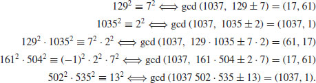
Three of them yield a factorization of .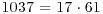

It is clear that the CFRAC factoring algorithm is essentially just a continued fraction algorithm for finding the continued fraction expansion [q0, q1, ···, qk, ···] of , or the Pk and Qk of such an expansion. In what follows, we shall briefly summarize the CFRAC method just discussed above in the following algorithmic form:

Algorithm 4.6 (CFRAC factoring) Given a positive integer n and a positive integer k such that kn is not a perfect square, this algorithm tries to find a factor of n by computing the continued fraction expansion of .

1. Let n be the integer to be factored and k any small integer (usually 1), and let the factor base, FB, be a set of small primes chosen such that it is possible to find some integer xi such that . Usually, FB contains all such primes less than or equal to some limit. Note that the multiplier k>1 is needed only when the period is short. For example, Morrison and Brillhart used k = 257 in factoring F7.

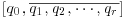2. Compute the continued fraction expansion of for a number of values of k. This gives us good rational approximations P/Q. The recursion formulas to use for computing P/Q are as follows:

This can be done by a continued fraction algorithm such as Theorem 2.26 introduced earlier.

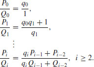
3. Try to factor the corresponding integer W = P2−Q2kn in our factor base FB. Since , each of these W is only about half the length of kn. If we succeed, we get a new congruence. For each success, we obtain a congruence

since, if Pi/Qi is the ith continued fraction convergent to and , then

(4.29)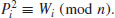

4. Once we have obtained at least m + 2 such congruences, then by Gaussian elimination over we obtain a congruence 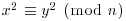. That is, if (x1, e01, e11, ···, em1), ···, (xr, e0r, e1r, ···, emr) are solutions of (4.24) such that the vector sum defined in (4.25) is even in each component, then

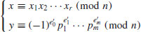
is a solution to , except for the possibility that , and hence we have

which are then possibly nontrivial factors of n.

Conjecture 4.3 (The complexity of the CFRAC Method) If n is the integer to be factored, then under certain reasonable heuristic assumptions, the CFRAC method will factor n in time

(4.30)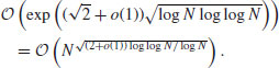

Remark 4.4 This is a conjecture, not a theorem, because it is supported by some heuristic assumptions which have not been proven.

Problems for Section 4.5

1. Let

be the continued fraction expansion of x. Find the successive convergents Pi/Qi of this continued fraction.

2. Let the successive convergents Pi/Qi of the continued fraction of x be as follows:

Find the continued fraction expansion of x.

3. Let n be a positive integer that is not a perfect square. Let Pk/Qk the kth convergent of the simple continued fraction expansion of . Then

4. Let

(4.31)

If

are solutions to (4.31) such that

then

is a solution to

5. Give a heuristic analysis of the running time of the CFRAC method

6. Implement the CFRAC algorithm on a computer.

7. Use your CFRAC program above to factor the integers 1037, 193541963, and 19354196373153173137.

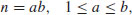
4.6 Quadratic Sieve

The idea of the quadratic sieve (QS) was first introduced by Carl Pomerance in 1982 [8]. QS is somewhat similar to CFRAC except that instead of using continued fractions to produce the values for , it uses expressions of the form

(4.32)

Here, if 0<k<L, then

(4.33)

If we get

(4.34)

then we have with

(4.35)

Once such x and y are found, there is a good chance that is a nontrivial factor of n.

Example 4.10 Use the Quadratic Sieve Method (QS) to factor n = 2041. Let W(x) = x2−n, with x = 43, 44, 45, 46. Then we have:

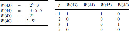
which leads to the following congruence:

This congruence gives the factorization of 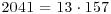, since

For the purpose of implementation, we can use the same set FB as that used in CFRAC and the same idea as that described above to arrange (4.34) to hold.

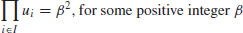
The most widely used variation of the quadratic sieve is perhaps the Multiple Polynomial Quadratic Sieve (MPQS), first proposed by Peter Montgomery in 1986. The idea of the MPQS is as follows: To find the (x, y) pair in

(4.36)

we try to find triples (Ui, Vi, Wi), for , such that

(4.37)

where W is easy to factor (at least easier than n). If sufficiently many congruences (4.37) are found, they can be combined, by multiplying together a subset of them, in order to get a relation of the form (4.36). The version of the MPQS algorithm described here is based on [9].

Algorithm 4.7 (Multiple Polynomial Quadratic Sieve) Given a positive integer n>1, this algorithm will try to find a factor n using the multiple polynomial quadratic sieve.

1. Choose B and M, and compute the factor base FB.

Note: M is some fixed integer so that we can define: U(x) = a2x + b, V = a and W(x) = a2x2 + 2bx + c, , such that a, b, c satisfy the following relations:

(4.38)

Note: The potential prime divisors p of a given quadratic polynomial W(x) may be characterized as: If , then

(4.39)

That is, the congruence should be solvable. So, the factor base FB (consisting of all primes less than a bound B) should be chosen in such a way that is solvable. There are L primes pj, in FB; this set of primes is fixed in the whole factoring process.

2. Generate a new quadratic polynomial W(x).

Note: The quadratic polynomial W(x) in

(4.40)

assumes extreme values in such that . If , then , thus W(x) is easier to factor than n.

3. Solve for all q = pe<B, for all primes , and save the solutions for each q.

4. Initialize the sieving array SI[−M, M) to zero.

5. Add log p to all elements SI(j), , for which , for all q = pe<B, and for all primes .

Note: Now we can collect those for which W(x) is only composed of prime factors <B.

6. Select those for which SI(j) is closed to .

7. If the number of W(x)-values collected in Step 6 is <L + 2, then go to Step 2 to construct a new polynomial W(x).

Note: If at least L + 2 completely factorized W-values have been collected, then the (x, y)-pairs satisfying (4.36) may be found as follows: For xi, ,

(4.41)

8. Perform Gaussian elimination on the matrix of exponents (mod 2) of W(x).

Note: Associated with each W(xi), we define the vector as follows

(4.42)

Since we have more vectors (at least L + 2) than components (L + 1), there exists at least one subset s of the set such that

(4.43)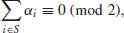

so that

(4.44)

Hence, from (4.40) it follows that

(4.45)

which is of the required form .

9. Compute .

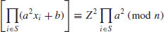
Note: Now we can calculate to find the prime factors of n.

Example 4.11 MPQS has been used to obtain many spectacular factorizations. One such factorization is the 103-digit composite number

The other record of the MPQS is the factorization of the RSA-129 in April 1994, a 129 digit composite number:

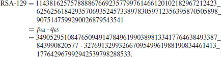
It was estimated in Gardner [23] in 1977 that the running time required to factor numbers with about the same size as RSA-129 would be about 40 quadrillion years using the best algorithm and fastest computer at that time. It was factorized by Derek Atkins, Michael Graff, Arjen Lenstra, Paul Leyland, and more than 600 volunteers from more than 20 countries, on all continents except Antarctica. To factor this number, they used the double large prime variation of the Multiple Polynomial Quadratic Sieve Factoring Method. The sieving step took approximately 5000 mips years.

Conjecture 4.4 (The complexity of the QS/MPQS Method) If n is the integer to be factored, then under certain reasonable heuristic assumptions, the QS/MPQS method will factor n in time

(4.46)

Problems for Section 4.6

1. Show that

2. Show that

3. Show that if n = pk with p prime and , then .

4. Let n = p1p2···pk, where are distinct odd primes. Let also . Then the congruence

has exact 2k solutions modulo n, two of them are

5. Let x and y be randomly chosen so that

Show that the chance of

is greater than 1/2. That is, the chance for

is greater than 1/2.

6. Find a suitable pair of integers (x, y) such that

and then factor 139511931371319137.

7. A number is smooth if all of its prime factors are small; a number is B-smooth if all of its prime factors are . Let the numbers of primes in the interval [1, B] and be positive B-smooth integers with . Show that some nonempty subset of has product which is a square.

8. Let be an arbitrary small positive integer, and

Show that if is chosen from [1, x] independently and uniformly, then the probability that some nonempty subset product is a square tends to 1 as , whereas the probability that some nonempty subset product is a square tends to 0 as if is chosen.

9. Let be y-smooth numbers up to x. Show that the expected number of choices of random integers in [1, x] to find one y-smooth number is

and to find such y-smooth numbers is

10. Let be y-smooth number, and let each be factored as follows

Show that

if and only if

as a vector in . Moreover, such a nontrivial subset is guaranteed amongst

11. Let be any fixed, positive real number. Show that

12. Deduce that the Quadratic Sieve is a deterministic factoring algorithm with the following conjectured complexity

4.7 Number Field Sieve

Before introducing the Number Field Sieve (NFS), it is interesting to briefly review some important milestones in the development of the factoring methods. In 1970, it was barely possible to factor “hard” 20-digit numbers. In 1980, by using the CFRAC method, factoring of 50-digit numbers was becoming commonplace. In 1990, the QS method had doubled the length of the numbers that could be factored by CFRAC, with a record having 116 digits. In the spring of 1996, the NFS method had successfully split a 130-digit RSA challenge number in about 15% of the time the QS would have taken. At present, the Number Field Sieve (NFS) is the champion of all known factoring methods. NFS was first proposed by John Pollard in a letter to A. M. Odlyzko, dated August 31 1988, with copies to R. P. Brent, J. Brillhart, H. W. Lenstra, C. P. Schnorr, and H. Suyama, outlining an idea of factoring certain big numbers via algebraic number fields. His original idea was not for any large composite, but for certain “pretty” composites that had the property that they were close to powers. He illustrated the idea with a factorization of the seventh Fermat number which was first factored by CFRAC in 1970. He also speculated in the letter that “if F9 is still unfactored, then it might be a candidate for this kind of method eventually?” The answer now is of course “yes,” since F9 was factored by using NFS in 1990. It is worthwhile pointing out that NFS is not only a method suitable for factoring numbers in a special form like F9, but also a general purpose factoring method for any integer of a given size. There are, in fact, two forms of NFS (Huizing [10], and Lenstra and Lenstra [11]): the special NFS (SNFS), tailored specifically for integers of the form N = c1rt + c2su, and the general NFS (GNFS), applicable to any arbitrary numbers. Since NFS uses some ideas from algebraic number theory, a brief introduction to some basic concepts of algebraic number theory is in order.

Definition 4.1 A complex number is an algebraic number if it is a root of a polynomial

(4.47)

where and . If f(x) is irreducible over and , then k is the degree of x.

Example 4.12 Two examples of algebraic numbers are as follows:

1. rational numbers, which are the algebraic numbers of degree 1.

2. , which is of degree 2 because we can take f(x) = x2−2 = 0 ( is irrational).

Any complex number that is not algebraic is said to be transcendental such as and e.

Definition 4.2 A complex number is an algebraic integer if it is a root of a monic polynomial

(4.48)

where .

Remark 4.5 A quadratic integer is an algebraic integer satisfying a monic quadratic equation with integer coefficients. A cubic integer is an algebraic integer satisfying a monic cubic equation with integer coefficients.

Example 4.13 Some examples of algebraic integers are as follows:

1. ordinary (rational) integers, which are the algebraic integers of degree 1. That is they satisfy the monic equations x−a = 0 for .

2. and , because they satisfy the monic equations x3−2 = 0 and x3−5 = 0, respectively.

3. , because it satisfies x2 + x + 1 = 0.

4. Gaussian integer , with .

Clearly, every algebraic integer is an algebraic number, but the converse is not true.

Proposition 4.1 A rational number is an algebraic integer if and only if .

Proof: If , then r is a root of x−r = 0. Thus r is an algebraic integer Now suppose that and r is an algebraic integer (i.e., r = c/d is a root of (4.48), where ; we may assume ). Substituting c/d into (4.48) and multiplying both sides by dn, we get

It follows that and (since ). Again since , it follows that . Hence . It follows, for example, that 2/5 is an algebraic number but not an algebraic integer.

Remark 4.6 The elements of are the only rational numbers that are algebraic integers. We shall refer to the elements of as rational integers when we need to distinguish them from other algebraic integers that are not rational. For example, is an algebraic integer but not a rational integer.

The most interesting results concerned with the algebraic numbers and algebraic integers are contained in the following theorem.

Theorem 4.2 The set of algebraic numbers forms a field, and the set of algebraic integers forms a ring.

Proof: See pp. 67–68 of Ireland and Rosen [12].

Lemma 4.1 Let f(x) be an irreducible monic polynomial of degree d over integers and M an integer such that . Let be a complex root of f(x) and the set of all polynomials in with integer coefficients. Then there exists a unique mapping satisfying

1. ;

2. ;

3. ;

4. ;

5. .

Now we are in a position to introduce the Number Field Sieve (NFS). Note that there are two main types of NFS: NFS (general NFS) for general numbers and SNFS (special NFS) for numbers with special forms. The idea, however, behind the GNFS and SNFS is the same:

1. Find a monic irreducible polynomial f(x) of degree d in , and an integer M such that .

2. Let be an algebraic number that is the root of f(x), and denote the set of polynomials in with integer coefficients as .

3. Define the mapping (ring homomorphism): via which ensures that for any , we have .

4. Find a finite set u of coprime integers (a, b) such that

(4.49)

for and . Let . Then

which is of the required form of the factoring congruence, and hopefully a factor of n can be found by calculating .

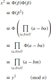
There are many ways to implement the above idea, all of which follow the same pattern as we discussed previously in CFRAC and QS/MPQS: By a sieving process one first tries to find congruences modulo n by working over a factor base, and then does a Gaussian elimination over to obtain a congruence of squares . We give in the following a brief description of the NFS algorithm [13].

Algorithm 4.8 Given an odd positive integer n, the NFS algorithm has the following four main steps in factoring n:

1. (Polynomials Selection) Select two irreducible polynomials f(x) and g(x) with small integer coefficients for which there exists an integer M such that

(4.50)

The polynomials should not have a common factor over .

2. (Sieving) Let be a complex root of f and a complex root of G. Find pairs (a, b) with such that the integral norms of and :

(4.51)

are smooth with respect to a chosen factor base. (The principal ideals and factor into products of prime ideals in the number field and , respectively.)

3. (Linear Algebra) Use techniques of linear algebra to find a set of indices such that the two products

(4.52)

are both squares of products of prime ideals.

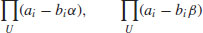
4. (Square Root) Use the set s in (4.52) to find algebraic numbers and such that

(4.53)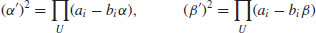

Define 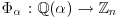and via , where M is the common root of both f and G. Then

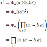
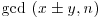
which is of the required form of the factoring congruence, and hopefully, a factor of n can be found by calculating .

Example 4.14 We first give a rather simple NFS factoring example. Let . So we put f(x) = x2 + 1 and m = 122, such that

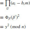
If we choose , then we can easily find (by sieving) that

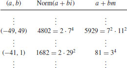
(Readers should be able to find many such pairs of (ai, bi) in the interval, that are smooth up to e.g., 29.) So, we have

Thus,

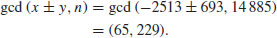
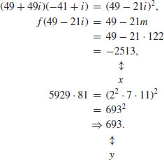
In the same way, if we wish to factor n = 84101 = 2902 + 1, then we let m = 290, and f(x) = x2 + 1 so that

We tabulate the sieving process as follows:

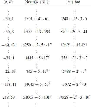
Clearly, −38 + i and −22 + 19i can produce a product square, since

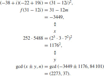
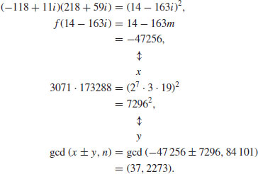
In fact, 84101 = 2273× 37. Note that −118 + 11i and 218 + 59i can also produce a product square, since

Example 4.15 Next we present a slightly more complicated example. Use NFS to factor n = 1098413. First notice that , which is in a special form and can be factored by using SNFS.

1. (Polynomials Selection) Select the two irreducible polynomials f(x) and g(x) and the integer M as follows:

2. (Sieving) Suppose after sieving, we get as follows:

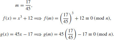
That is, the chosen polynomial that produces a product square can be constructed as follows (as an exercise, readers may wish to choose some other polynomial which can also produce a product square):

Let and . Then

So, we get the required square of congruence:

Thus,

That is,

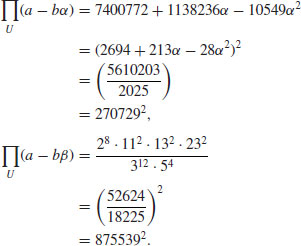
Example 4.16 Finally, we give some large factoring examples using NFS.

1. SNFS examples: One of the largest numbers factored by SNFS is

It was announced by P. Montgomery, S. Cavallar, and H. te Riele at CWI in Amsterdam on September 3 1997. They used the polynomials f(x) = x5−144 and g(x) = 1233x + 1 with common root . The factor base bound was 4.8 million for f and 12 million for G. Both large prime bounds were 150 million, with two large primes allowed on each side. They sieved over million and million. The sieving lasted 10.3 calendar days; 85 SGI machines at CWI contributed a combined 13027719 relations in 560 machine-days. It took 1.6 more calendar days to process the data. This processing included 16 CPU-hours on a Cray C90 at SARA in Amsterdam to process a 1969262× 1986500 matrix with 57942503 nonzero entries. The other large number factorized by using SNFS is the 9th Fermat number:

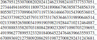
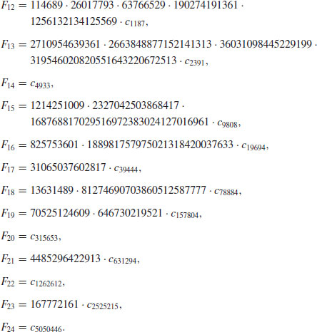
a number with 155 digits; it was completely factored in April 1990. The most wanted factoring number of special form at present is the 12th Fermat number ; we only know its partial prime factorization:

and we want to find the prime factors of the remaining 1187-digit composite.

2. GNFS examples: Three large general numbers RSA-130 (in April 1996), RSA-140 (in February 1999), RSA-155 (August 1999), and RSA-174 (December 2003) were factorized using GNFS:

Remark 4.7 Prior to the NFS, all modern factoring methods had an expected running time of at best

For example, Dixon’s Random Square Method has the expected running time

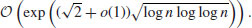
whereas the Multiple Polynomial Quadratic Sieve (MPQS) takes time

Because of the Canfield-Erdös-Pomerance theorem, some people even believed that this could not be improved upon except maybe for the term (c + o(1)), but the invention of the NFS has changed all this.

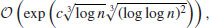
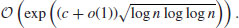
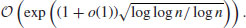
Conjecture 4.5 (Complexity of NFS) Under some reasonable heuristic assumptions, the NFS method can factor an integer n in time

(4.54)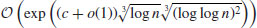

where if GNFS is used to factor an arbitrary integer n, whereas if SNFS is used to factor a special integer n.

Problems for Section 4.7

1. (General Factoring Challenge Problems) Try to complete the prime factorization, either individually or in group, of the following RSA challenge numbers (Note that in these numbers, the value for x in RSA-x represents the number of bits, not the number of digits; this is just the RSA convention for these numbers):

2. (Knuth’s Factoring Challenge Problem) Knuth in 1998 proposed the following 211 digits factoring challenge number [4], marked its difficulty degree as 50, one of the hardest problems in his book:

Try to complete the prime factorization, either individually or in group, of the above Knuth factoring challenge number.

3. (Rivest’s Factoring Challenge Problem) In April 1999, when the MIT Laboratory for Computer Science celebrated its 35 anniversary, Prof Ron Rivest proposed the following factoring challenge problem as a part of his Secret-Key Computing Challenge Problem:

Try to complete the prime factorization, either individually or in group, of the above Rivest’s factoring challenge number.

4. In this problem, we list the smallest unfactored (not completely factored) Fermat numbers for you to try to find the complete factorization for each of these numbers:

4.8 Bibliographic Notes and Further Reading

In this chapter, we discussed some of the most popular algorithms for integer factorization. For general references in this field, it is suggested that readers consult, for example, [14–38].

Shanks’ Square Forms Factorization was studied in [39]. The p−1 Factoring Method was proposed by Pollard in [40] and Factoring Method in [2], respectively. An improved version of was proposed by Brent in [3]. The p + 1 Factoring Method was proposed by Williams in [41].

The ECM factoring method was first proposed by Lenstra in [42]. More information on ECM may be found in [5,6]. The CFRAC factoring method was first proposed and implemented in [7]. The QS factoring method was first proposed by Pomerance in the 1980s [9, 43,44]. The idea of NFS was first proposed by Pollard and subsequently improved by many authors; more information about the NFS can be found in [11, 45,46]. Readers who are interested in parallel and distributed factoring may consult [47–50].

References

1. P. Shor, “Polynomial-Time Algorithms for Prime Factorization and Discrete Logarithms on a Quantum Computer”, SIAM Journal on Computing, 26, 5, 1997, pp. 1484–1509.

2. J. M. Pollard, “A Monte Carlo Method for Factorization”, BIT, 15, 1975, pp. 331–332.

3. R. P. Brent, “An Improved Monte Carlo Factorization Algorithm”, BIT, 20, 1980, pp. 176–184.

4. D. E. Knuth, The Art of Computer Programming II – Seminumerical Algorithms, 3rd Edition, Addison-Wesley, 1998.

5. P. L. Montgomery, “Speeding Pollard’s and Elliptic Curve Methods of Factorization”, Mathematics of Computation, 48, 1987, pp. 243–264.

6. R. P. Brent, “Some Integer Factorization Algorithms using Elliptic Curves”, Australian Computer Science Communications, 8, 1986, pp. 149–163.

7. M. A. Morrison and J. Brillhart, “A Method of Factoring and the Factorization of F7”, Mathematics of Computation, 29, 1975, pp. 183–205.

8. C. Pomerance, “Analysis and Comparison of some Integer Factoring Algorithms”, in H. W. Lenstra, Jr. and R. Tijdeman, eds, Computational Methods in Number Theory, No 154/155, Mathematical Centrum, Amsterdam, 1982, pp. 89–139.

9. H. J. J. te Riele, W. Lioen, and D. Winter, “Factoring with the Quadrtaic Sieve on Large Vector Computers”, Journal of Computational and Applied Mathematics, 27, 1989, pp. 267–278.

10. R. M. Huizing, “An Implementation of the Number Field Sieve”, Experimental Mathematics, 5 3, 1996, pp. 231–253.

11. A. K. Lenstra and H. W. Lenstra, Jr. (editors), The Development of the Number Field Sieve, Lecture Notes in Mathematics 1554, Springer-Verlag, 1993.

12. K. Ireland and M. Rosen, A Classical Introduction to Modern Number Theory, 2nd Edition, Graduate Texts in Mathematics 84, Springer, 1990.

13. P. L. Montgomery, “A Survey of Modern Integer Factorization Algorithms”, CWI Quarterly, 7, 4, 1994, pp. 337–394.

14. L. M. Adleman, “Algorithmic Number Theory – The Complexity Contribution”, Proceedings of the 35th Annual IEEE Symposium on Foundations of Computer Science, IEEE Press, 1994, pp. 88–113.

15. D. Atkins, M. Graff, A. K. Lenstra, and P. C. Leyland, “The Magic Words are Squeamish Ossifrage”, Advances in Cryptology – ASIACRYPT’94, Lecture Notes in Computer Science 917, 1995, pp. 261–277.

16. R. P. Brent, “Primality Testing and Integer Factorization”, Proceedings of Australian Academy of Science Annual General Meeting Symposium on the Role of Mathematics in Science, Canberra, 1991, pp. 14–26.

17. R. P. Brent, “Recent Progress and Prospects for Integer Factorization Algorithms”, Proc. COCOON 2000 (Sydney, July 2000), Lecture Notes in Computer Science 1858, Springer, 2000, pp. 3–22.

18. D. M. Bressound, Factorization and Primality Testing, Springer, 1989.

19. H. Cohen, A Course in Computational Algebraic Number Theory, Graduate Texts in Mathematics 138, Springer-Verlag, 1993.

20. T. H. Cormen, C. E. Ceiserson and R. L. Rivest, Introduction to Algorithms, 3rd Edition, MIT Press, 2009.

21. R. Crandall and C. Pomerance, Prime Numbers – A Computational Perspective, 2nd Edition, Springer-Verlag, 2005.

22. J. D. Dixon, “Factorization and Primality tests”, The American Mathematical Monthly, June–July 1984, pp. 333–352.

23. M. Gardner, “Mathematical Games – A New Kind of Cipher that Would Take Millions of Years to Break”, Scientific American, 237, 2, 1977, pp. 120–124.

24. C. F. Gauss, Disquisitiones Arithmeticae, G. Fleischer, Leipzig, 1801. English translation by A. A. Clarke, Yale University Press, 1966. Revised English translation by W. C. Waterhouse, Springer-Verlag, 1975.

25. A. Granville, “Smooth Numbers: Computational Number Theory and Beyond”, Algorithmic Number Theory. Edited by J. P. Buhler and P. Stevenhagen, Cambridge University Press, 2008, pp. 267–323.

26. T. Kleinjung, et al., “Factorization of a 768-Bit RSA Modulus”, In: T. Rabin (Ed.), CRYPTO 2010, Lecture Notes in Computer Science 6223, Springer, 2010, pp. 333–350.

27. N. Koblitz, A Course in Number Theory and Cryptography, 2nd Edition, Graduate Texts in Mathematics 114, Springer-Verlag, 1994.

28. A. K. Lenstra, “Integer Factoring”, Design, Codes and Cryptography, 19, 2/3, 2000, pp. 101–128.

29. R. A. Mullin, Algebraic Number Theory, 2nd Edition, CRC Press, 2011.

30. C. Pomerance “Integer Factoring”, Cryptology and Computational Number Theory. Edited by C. Pomerance, Proceedings of Symposia in Applied Mathematics, American Mathematical Society, 1990, pp. 27–48.

31. C. Pomerance, “On the Role of Smooth Numbers in Number Theoretic Algorithms”, Proceedings of the Intenational Congress of Mathematicians, Zurich, Switzerland 1994, Birkhauser Verlag, Basel, 1995, pp. 411–422.

32. C. Pomerance, “A Tale of Two Sieves”, Notice of the AMS, 43, 12, 1996, pp. 1473–1485.

33. H. Riesel, Prime Numbers and Computer Methods for Factorization, Birkhäuser, Boston, 1990.

34. V. Shoup, A Computational Introduction to Number Theory and Algebra, Cambridge University Press, 2005.

35. H. C. Williams, “The Influence of Computers in the Development of Number Theory”, Computers & Mathematics with Applications, 8, 2, 1982, pp. 75–93.

36. H. C. Williams, “Factoring on a Computer”, Mathematical Intelligencer, 6, 3, 1984, pp. 29–36.

37. S. Y. Yan, “Computing Prime Factorization and Discrete Logarithms: From Index Calculus to Xedni Calculus”, International Journal of Computer Mathematics, 80, 5, 2003, pp. 573–590.

38. S. Y. Yan, Primality Testing and Integer Factorization in Public-Key Cryptography, Advances in Information Security 11, 2nd Edition, Springer, 2009.

39. S. McMath, Daniel Shanks’ Square Forms Factorization, United States Naval Academy, Annapolis, Maryland, 24 November 2004.

40. J. M. Pollard, “Theorems on Factorization and Primality Testing”, Procedings of Cambridge Philosophy Society, 76, 1974, pp. 521–528.

41. H. C. Williams, “A p + 1 Method of Factoring”, Mathematics of Computation, 39, 1982, pp. 225–234.

42. H. W. Lenstra, Jr., “Factoring Integers with Elliptic Curves”, Annals of Mathematics, 126, 1987, pp. 649–673.

43. C. Pomerance, “The Quadratic Sieve Factoring Algorithm”, Proceedings of Eurocrypt 84, Lecture Notes in Computer Science 209, Springer, 1985, pp. 169–182.

44. C. Pomerance, “Smooth Numbers and the Quadratic Sieve”, Algorithmic Number Theory. Edited by J. P. Buhler and P. Stevenhagen, Cambridge University Press, 2008, pp. 69–81.

45. C. Pomerance, “The Number Field Sieve”, Mathematics of Computation, 1943–1993, Fifty Years of Computational Mathematics. Edited by W. Gautschi, Proceedings of Symposium in Applied Mathematics 48, American Mathematical Society, Providence, 1994, pp. 465–480.

46. P. Stevenhagen, “The Number Field Sieve”, Algorithmic Number Theory. Edited by J.P. Buhler and P. Stevenhagen, Cambridge University Press, 2008, pp. 83–100.

47. R. P. Brent, “Parallel Algorithms for Integer Factorisation”, Number Theory and Cryptography. Edited by J. H. Loxton, London Mathematical Society Lecture Notes i 154, Cambridge University Press, 1990, pp. 26–37.

48. R. P. Brent, “Some Parallel Algorithms for Integer Factorisation”, Proceedings of 5th International Euro-Par Conference(Toulouse, France), Lecture Notes in Computer Science 1685, Springer, 1999, pp. 1–22.

49. A. K. Lenstra and M. S. Manases “Factoring by Electronic Mail”, Advances in Cryptology – EUROCRYPT Ô89. Edited by J. J. Quisquater and J. Vandewalle, Lecture Notes in Computer Science 434, Springer, 1990, pp. 355–371.

50. R. D. Silverman, “Massively Distributed Computing and Factoring Large Integers”, Communications of the ACM, 34, 11, 1991, pp. 95–103.