2
Strain
2.1. Notion of strain
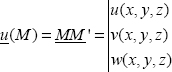
2.1.1. Displacement vector
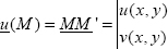
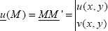
Let us say that S is a solid and M(x, y, z) is a point of S. Under the action of external forces, S becomes S’ and M becomes M’. This is called the displacement vector of the point M, and we note u(M), the vector MM’.
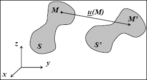
2.1.2. Unit strain
Thus, there are two points of S: M and N, which are displaced to M’ and N’ after stress and n the unit vector:


Figure 2.2. Unit strain. For a color version of this figure, see www.iste.co.uk/bouvet/aeronautical.zip
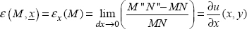
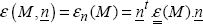
This is called unit strain in M according to n:
Evidently, ε(M,n) has no unit.
This strain ε(M, n) must remain small in front of one in order to belong within the Small Perturbation Hypothesis (SPH).
As indicated by its name, this hypothesis translates the length strain of the matter in the n-direction.
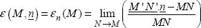
In particular, if n is equal to x, and the relation is put in 2D in order to facilitate representations:
Figure 2.3. Unit strain formula. For a color version of this figure, see www.iste.co.uk/bouvet/aeronautical.zip
As N(x + dx, y) is close to M(x, y), we have:
And
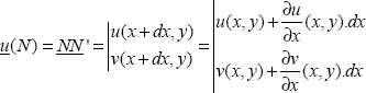
Hence:
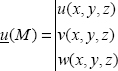
Evidently in 3D, we can make the following displacement generalization for a point M(x, y, z):
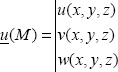
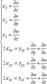
These strains are defined according to the x-, y- and z- directions by:
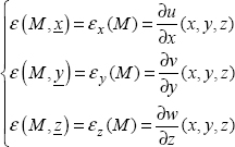
And εx, εy and εz therefore translate the length strain of the matter in the x-, y-, and z-directions, respectively.
2.1.3. Angular distortion
As defined by the figure above, M is one point and M1 and M2 are two points that are close to M, which are displaced to M’, M1’ and M2’ respectively.
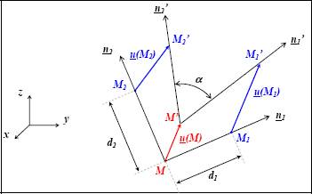
Figure 2.4. Angular distortion. For a color version of this figure, see www.iste.co.uk/bouvet/aeronautical.zip
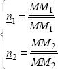
The two unit vectors are defined as:
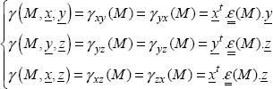
According to n1 and n2, the angular distortion is at M:
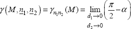
Evidently, γ(M, n1, n2) has no unit.
This strain γ(M, n1, n2) must remain small in front of one in order to belong within the SPH.
It translates the angle variation of the matter, called shear, of the angle that was initially a right-angled corner (n1, n2). Altogether, the larger the distortion, less right-angled the corner will be.
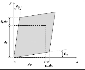
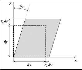
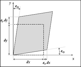
In particular, if n1 is equal to x, if n2 is equal to y, and placed in 2D in order to facilitate the representations:
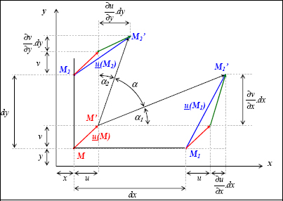
Figure 2.5. Angular distortion formula. For a color version of this figure, see www.iste.co.uk/bouvet/aeronautical.zip
As M1(x + dx, y) and M2(x, y + dy) are close to M(x, y), we have:
And:
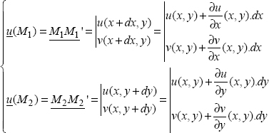
Yet:
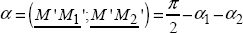
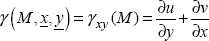
Hence:
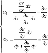
And:
Evidently in 3D, we can make a generalization for point M(x, y, z), for which the displacement is worth:
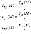
The angular distortions are therefore defined by:
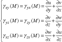
Therefore, (with i and j as variants of 1–3, and i being different to j) we evidently have:

yxy, Yyz and yxz therefore translate the angle variation of the matter for the angles which were initially right-angled corners: (x, y), (y, z) and (z, x), respectively.
2.2. Strain matrix
2.2.1. Definition of the strain matrix
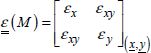
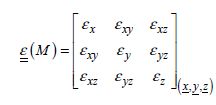
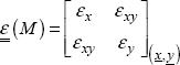
The following matrix is called the strain matrix  :
:
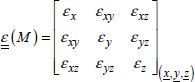
With (be careful here):
This matrix is therefore obviously symmetrical.
Based on the displacement field, it is defined by the relations seen previously:
Or, in the tensorial form:
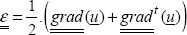
The benefit of using the tensorial form is of course that it remains true for every coordinate system (Cartesian, cylindrical or spherical), in contrast to the previous form, which is only true in Cartesian coordinates. All the same, the displacement gradient of the coordinate system in question remains to be determined.
EXAMPLES: DRAWING THE 2D STRAINS.–
A small square is subjected to the strain tensor:
It is strained in the following way:
This drawing may be simple and basic but it is essential to interpret the strain tensor. Moreover, it is only valid for SPH.
Finally, it is defined at a close translation and rotation. Indeed, two displacement fields, which differ from a rigid body displacement field, produce the same strain. Therefore, we could have represented this diagram in the following form:
The strain tensor enables us to completely characterize the state of a strain of a material point. In particular, it enables us to easily find the unit strain in any direction, or the angular distortion of two orthogonal vectors.
As a matter of fact, it can be shown that:
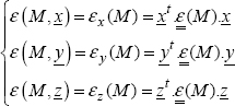
And, whatever the vector n is, the strain in this direction is worth:
Likewise:
And therefore, whatever the n and t orthogonal vectors, the distortion according to n and t is worth:

We will notice that these two relations of the strains are very similar to the relations which enable us to determine the normal and shear stresses:
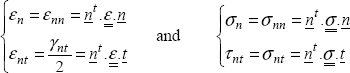
These four relations are very practical to determine the strains, the angular distortions, the normal stresses or the shear stresses in any direction (or coordinate system), and summarize the use of stress tensors and strain tensors.
Note that εn and εnn are simply two different notations for speaking about the same thing, just the same as σn and σnn or τnt and σnt.
2.2.2. Principal strains and principal directions
As the 3D strain matrix is:
We can evidently determine this strain matrix in (x1, y1, z1) by:
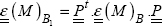
with  , the rotation matrix from the basis B to the basis B1, representing the vector coordinates of B1 expressed in the basis B.
THEOREM.– There is a direct orthonormal coordinate system (xI, xII, xIII) in which the strain matrix is diagonal:
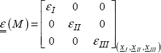
εI εII, and εIII are called principal strains and xI, xII and xIII are called principal directions , which are associated with εI, εII and εIII, respectively.
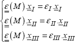
We then clearly have:
And in practical terms, to determine the principal strains, it is sufficient to write:
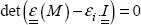
which gives three solutions (or two in 2D). Then, to determine the three principal directions, it is sufficient to write the three previous relations.
This can be translated by the following drawing:
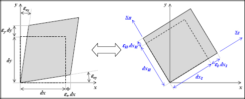
Figure 2.8. Strain of a square and principal strains. For a color version of this figure, see www.iste.co.uk/bouvet/aeronautical.zip
As seen by the matter on these two diagrams, the state of strain is the same.
EXAMPLES: SHEAR.–
As the strain tensor is:
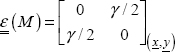
Hence, we can show that the principal strains are +γ/2 and –γ/2 and the principal directions are oriented at +45° and −45°:
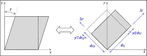
Figure 2.9. Strain of a square and principal strains in pure shear. For a color version of this figure, see www.iste.co.uk/bouvet/aeronautical.zip
This result can be easily understood on a physical level, as we can easily use our hands to feel that the applied force on the left diagram pulls at +45° and compresses at −45°.
This result is similar to that found for shear stresses. As a matter of fact, for isotropic materials, the shear stress simply causes shear strain.
2.2.3. Volume expansion
If we calculate the variation of a small rectangular section subjected to plane strain, we then find:
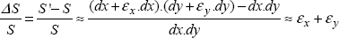
The area variation is therefore equal to the trace of the 2D strain tensor. Evidently, this result is only true within the SPH.
The result is similar in 3D:
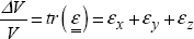
Physically, as this volume variation is the same, regardless of the coordinate system in which the strain matrix is written, the trace must therefore be an invariant of the strain tensor, which is clearly the case.
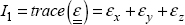
2.2.4. Invariants of strain tensor
Just as for the stress tensor, the strain tensor has three elementary invariants. Classically, we use:
- – the strain trace :
- – the von Mises strain :
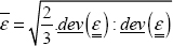
with the strain deviator, which is written as:
NOTE.– In order to find the equivalent plastic strain in plasticity and traction that is equal to the plastic strain in traction, the 2/3 coefficient is used instead of the 3/2 coefficient for the stress.
- – the determinant:

These invariants are far less common than for stresses, as the criteria are generally written on the basis of the stresses.
2.2.5. Compatibility condition
The strain field is derived from the displacement field:
Therefore, in order for the strain field to be integrable, it must verify the following condition:

This relation, called the strain compatibility condition, is very important if we are looking to solve a problem based on the stress method (see Chapter 4). These are some of the fundamental equations that a strain field needs to verify in order to be the solution to a problem (see Chapter 4).
2.3. Strain measurement: strain gage
In order to measure the strains in a solid, we use strain gages, which are resistances stuck onto the surface. If the solid becomes strained, the resistance varies, and we can then determine the strain as seen by the material.
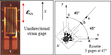
Figure 2.11. Unidirectional gage and rosette: three gages oriented at 45°. For a color version of this figure, see www.iste.co.uk/bouvet/aeronautical.zip
The size of a gage can vary from 1 to about 100 mm. The active parts are the bonded threads (the grid) in which the resistance is going to vary.
We can then determine the strain in the direction of the threads, and in that alone. We often use rosettes with three gages at 45°, which enable us to determine the three strains in the plane.
As a gage is stuck to a surface, it therefore only enables us to measure the plane strains:
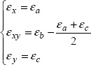
In practical terms, knowing the strains ɛa, ɛb and ɛc of a three-gage rosette at 45° (see the previous figure), it is sufficient to write that the strain, in the directions of the three gages given by the strain tensor, is equal to the strains given by the gages:
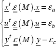
With:

Hence:
The gages are reliable and not very expensive, so they are widely used at present.
Moreover, in practice, it is almost impossible to measure the stress, so we generally settle for estimating them based on external forces. This estimation is thus based on stress distribution hypotheses, which can be marred by error.
Strain gages are therefore the best way to measure the strain of a structure. If we know the behavior law (see the next chapter) of the material, the stresses can be determined based on the strain. Due to malapropism, strain gage is incidentally often called stress gage!