3
Behavior Law
3.1. A few definitions
- – Behavior law: this is the relation that links the stress and strain. Evidently, it depends on the material and the external conditions (temperature, hygrometry, etc.).
- – Homogeneous: a material is said to be homogeneous if it behaves the same behavior at each point. In practice, it is never evidently neither completely true nor false. For example, a folded metal sheet will have different behavior in the area of folding as the material will have a different history.
- – Isotropic: a material is said to be isotropic if it behaves in the same way in all directions. In practice, it is never evidently neither completely true nor false. For example, a laminated metal sheet will have different behavior in its plane and in accordance with the normal direction as the lamination will have hardened (see section 3.3) this direction more substantially than the other two directions.
In this course, we will (almost) restrict ourselves to isotropic homogeneous materials.
3.2. Tension test
This is a sample with an applied force in tension:
We measure the tension stress σx based on the force F by:
and we measure the strains εx and εy based on two strain gages.
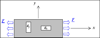
Figure 3.1. Tension test. For a color version of this figure, see www.iste.co.uk/bouvet/aeronautical.zip
3.2.1. Brittle materials
Brittle materials are: glass, ceramics, carbon, composites based on glass or carbon fibers, steels with a high elastic limit, etc.
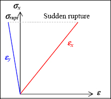
Figure 3.2. Tensile test of a brittle material. For a color version of this figure, see www.iste.co.uk/bouvet/aeronautical.zip
Quasi-linear curves are obtained until there is a sudden rupture. This behavior is linear elastic; elastic as in it all returns to its point of departure. As a matter of fact, we can find materials with nonlinear elastic behavior (rubber, etc.).
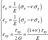
So, we adopt a linear elastic behavior law model:
with E being Young’s modulus (in MPa). For example, 210 GPa for the steel, 60 GPa for the glass, 200 GPa for the carbon and ν for Poisson’s ratio (without a unit), which is typically equal to about 0.3 for “standard” materials.
Be careful, you must bear in mind that this is just a behavior model; in other words, we observe that the curves are quasi-linear, so we model them with a refined law. However, this is just a model and in reality, behavior is always much more complex.
3.2.2. Ductile materials
Ductile materials are mainly metals: steel, copper, aluminum, etc.
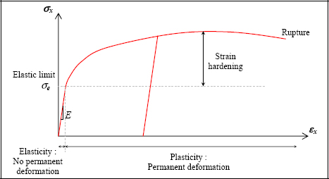
Figure 3.3. Tension test of a ductile material. For a color version of this figure, see www.iste.co.uk/bouvet/aeronautical.zip
We obtain a curve with a linear elastic beginning, then the rest of the curve is substantially nonlinear with a plasticity; plasticity in the sense where when discharging, it does not return to the point of departure and a permanent deformation is maintained under zero stress.
We can therefore adopt a linear behavior law if, and only if, the stress remains lower than the elastic limit:

- – if not, we define a behavior law with plasticity.
3.2.3. Particular cases
Be careful, you must bear in mind that these behavior laws are but models which pale in comparison to reality, which is always much more complex when looked at closely.
And even when one does not look too closely, there are certain behaviors which are more complex. For example, rubbers are elastic but substantially nonlinear; polymers are substantially viscous (they are a kind of intermediate between solids and liquids).
3.3. Shear test
This is a sample with an applied force in shear:
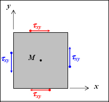
Figure 3.4. Shear. For a color version of this figure, see www.iste.co.uk/bouvet/aeronautical.zip
Evidently, the problem is much more complicated than applying a force to a material in tension. In practice, we use a cylinder with an applied force of torsion on a thin wall. It can therefore be shown that the applied force is mainly in shear stress (τzθ) and that it is homogeneous. We can therefore make an estimate based on the measurement of the torsion torque. The shear strain (γzθ) therefore remains to be determined, which is based on the strain gages stuck to the external wall (we can show that the gages at +45° and −45° fit the bill).

Figure 3.5. Torsion test. For a color version of this figure, see www.iste.co.uk/bouvet/aeronautical.zip
3.3.1. Brittle materials
We obtain quasi-linear curves until a sudden rupture. This behavior is linear elastic. We therefore adopt a linear elastic behavior law:
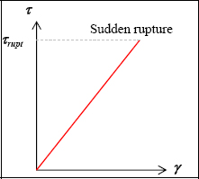
Figure 3.6. Brittle material shear test. For a color version of this figure, see www.iste.co.uk/bouvet/aeronautical.zip
with G being the shear modulus (in MPa). And for an isotropic linear elastic material, we can show that:
3.3.2. Ductile materials
Just as in the previous instance, we obtain a curve with an elastic beginning, and then the rest is plastic.
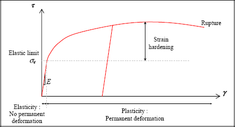
Figure 3.7. Shear test of a ductile material. For a color version of this figure, see www.iste.co.uk/bouvet/aeronautical.zip
We can therefore adopt a linear behavior law if, and only if, the stress remains lower than the elastic limit:
- – If τ < τe τ = G.γ
- – If not, we define a behavior law with plasticity.
And we experimentally take note that τe is approximately equal to half of σe.
3.4. General rule
3.4.1. Linear elasticity
Let us begin with 2D. If we give ourselves:
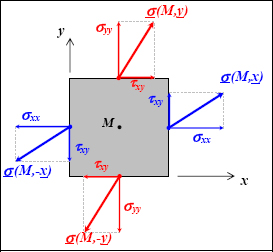
Figure 3.8. Stress vectors on the faces of a square. For a color version of this figure, see www.iste.co.uk/bouvet/aeronautical.zip
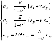
So, in the linear part (before any possible plasticity), we adopt an isotropic linear elastic behavior:
Or by reversing:
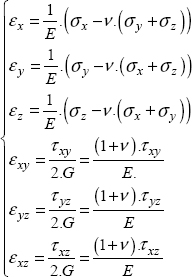
And in 3D:
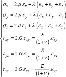
Or by reversing:
With λ and μ the Lamé parameters:
Or even more simply written in tensorial form:
This relation is fundamental, as it translates the relationship between stress and strain (in other words, it allows us to see whether the material is rigid or not). It is one of the fundamental equations that must verify the stress/strain fields in order to be the solution to the problem (see Chapter 4).
If we reverse this relation, we then find:
And by making some calculations, we can find the Lamé parameters by identifying these two relations.
EXAMPLES: VOLUME VARIATION IN TENSION.–
It can be shown that in tension:
And therefore:
The variation of volume is therefore:
And as ν is generally more or less equal to 0.3, we observe that the volume increases in a tension test.
EXAMPLES: FREE EXTERNAL SURFACE.–
On an external surface, with a normal ẕ, which is free from stress, we have:
The stress tensor is therefore in this form:
This is called a plane stress. To put it plainly, there is no stress vector outside the plane that is exerted on this external surface.
However, we can show that for an isotropic linear elastic material, strains are therefore in the form below:
With:
In other words, we can never have plane stress and plane strain at the same time.
In practice, in order to simplify problems, where possible, we try to position themselves in plane stress or plane strain. Evidently, these are only the hypotheses that remain to be verified or which have been verified based on previous experiments.
For example, if we study a thin plate, it can be shown that the stresses are planes on the two external surfaces, so at first approximation, they will be so in practice as well. And in this case, the strain will not then be plane.
On the other hand, if we study a thick plate, we can show that the plane strain hypothesis will be better suited to the problem. And in this case, the stress will not then be plane.
3.5. Anisotropic materials: example of a composite
So that you do not being to think that all materials are isotropic, we will now study a particular material, a composite made up of 50% (in volume) carbon fibers and 50% epoxy resin. This is classically used in aeronautics; it is T300/914. It is in the form of a 0.1 to 0.2 mm thick fabric which we will later cut, and then drape, in order to obtain the desired thickness.
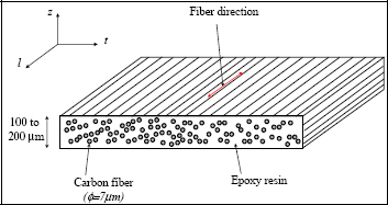
Figure 3.9. Unidirectional composite carbon/epoxy. For a color version of this figure, see www.iste.co.uk/bouvet/aeronautical.zip
3.5.1. Elasticity
Let us put the laminate plane in 2D (l, t); l for longitudinal and t for transversal directions. If we perform a tension test with the fibers in the θ-direction, we evidently note that the elasticity modulus depends on θ:

Figure 3.10. Young’s modulus of a UD composite versus the tension direction. For a color version of this figure, see www.iste.co.uk/bouvet/aeronautical.zip
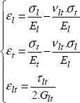
We can therefore simply write the behavior law in the coordinate (l, t):
Evidently, this is a little more complicated in (x, y). And for the T300/914 considered, we have:
3.6. Thermoelasticity
In the instance where the temperature of a free stress structure varies, we evidently observe thermal expansion phenomena. At first approximation, this expansion is translated by the strain that is proportional to this temperature variation:
where α is the coefficient of thermal expansion (in K−1), and the identity tensor signifies that the strain is homogeneous in every direction (if this strain is not constrained).
In order to factor in this thermally originated strain in elasticity, it is sufficient to add it to the elastic strain:
And the previous behavior relation remains valid if it is written with the elastic strain, and no longer with the total strain:
And by reversing it:
Or even:
EXAMPLES: CONSTRAINED OR FREE EXPANSION.–
If we consider a material that is free from stress and subjected to a temperature variation, which is placed in 2D:
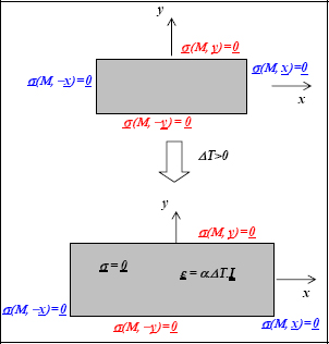
Figure 3.11. Thermal expansion with free stress. For a color version of this figure, see www.iste.co.uk/bouvet/aeronautical.zip
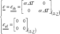
We can therefore show that the stress is homogeneous and null:
And that the structure is therefore subjected to a homogeneous strain field:
However, if we consider that the displacement is constrained:
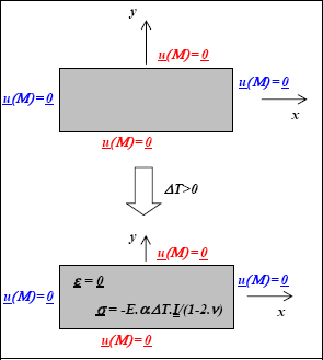
Figure 3.12. Thermal expansion with constrained strain. For a color version of this figure, see www.iste.co.uk/bouvet/aeronautical.zip
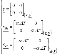
We can therefore show that the total strain is homogeneous and null, and that the elastic and thermal strains will balance each other out:
The structure is therefore subjected to a homogeneous bi-axial compression stress field:
Any readers who are interested may find details of these calculations in the exercise chapter (Beam thermal expansion: mono-material beam).


