Chapter 10: Worksheet Basics
Add a Worksheet
By default, when you create a new blank workbook in Excel, it contains one worksheet, which may be adequate. In some cases, however, your workbook might require additional worksheets in which to enter more data. For example, if your workbook contains data about products your company sells, you might want to add worksheets for each product category. You can easily add worksheets to a workbook.
When you add a new worksheet, Excel gives it a default name. To help you better keep track of your data, you can rename your new worksheet. For more information, see the next section, “Name a Worksheet.”
Add a Worksheet

 Click the Insert Worksheet button (
 ).
).
You can also right-click a worksheet tab and click Insert to open the Insert dialog box, where you can choose to insert a worksheet.

A Excel adds a new blank worksheet and gives it a default worksheet name.
Name a Worksheet
When you create a new workbook, Excel assigns default names to each worksheet in the workbook. Likewise, Excel assigns a default name to each worksheet you add to an existing workbook. (For more information about adding worksheets to a workbook, refer to the previous section, “Add a Worksheet.”)
To help you identify their content, you can change the names of your Excel worksheets to something more descriptive. For example, if your workbook contains four worksheets, each detailing a different sales quarter, then you can give each worksheet a unique name, such as Quarter 1, Quarter 2, and so on.
Name a Worksheet

Double-click the worksheet tab that you want to rename.
Excel highlights the current name.
You can also right-click the worksheet name and click Rename.
 Type a new name for the worksheet.
 Press
Press  .
.
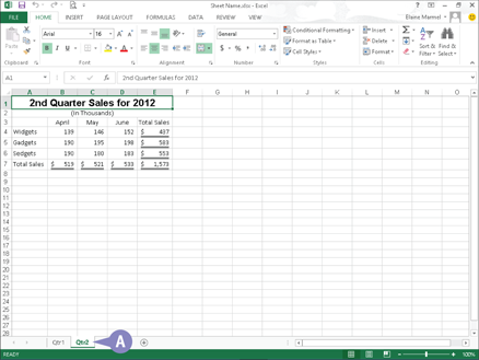
A Excel assigns the new worksheet name.
Change Page Setup Options
You can change worksheet settings related to page orientation, margins, paper size, and more. For example, suppose that you want to print a worksheet that has a few more columns than will fit on a page in Portrait orientation. (Portrait orientation accommodates fewer columns but more rows on the page and is the default page orientation that Excel assigns.) You can change the orientation of the worksheet to Landscape, which accommodates more columns but fewer rows on a page.
You can also use Excel’s page-setup settings to establish margins and insert page breaks to control the placement of data on a printed page.
Change Page Setup Options
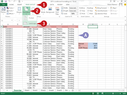
Change the Page Orientation
A Dotted lines identify page breaks that Excel inserts.
Click the Page Layout tab.
Click Orientation.
Click Portrait or Landscape.
Note: Portrait is the default orientation.

Excel applies the new orientation. This example applies Landscape.
B Excel moves the page break indicator based on the new orientation.
C You can click the Margins button to set up page margins.
Insert a Page Break

Select the row above which you want to insert a page break.
Click the Page Layout tab.
Click Breaks.
 Click Insert Page Break.

D Excel inserts a solid line representing a user-inserted page break.
Move and Copy Worksheets
You can move or copy a worksheet to a new location within the same workbook, or to an entirely different workbook. For example, moving a worksheet is helpful if you insert a new worksheet and the worksheet tab names appear out of order. Or, you might want to move a worksheet that tracks sales for the year to a new workbook so that you can start tracking for a new year.
In addition to moving worksheets, you can copy them. Copying a worksheet is helpful when you plan to make major changes to the worksheet.
Move and Copy Worksheets

If you plan to move a worksheet to a different workbook, open both workbooks and select the one containing the worksheet you want to move.
Click the tab of the worksheet you want to move or copy to make it the active worksheet.
Click the Home tab.
Click Format.
 Click Move or Copy Sheet.
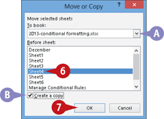
The Move or Copy dialog box appears.
A You can click  to select a workbook for the worksheet.
 Click the location where you want to place the worksheet that you are moving.
Note: Excel moves or copies sheets in front of the sheet you select.
B You can copy a worksheet by selecting Create a copy ( changes to
  ).
).
 Click OK.
Excel moves or copies the worksheet to the new location.
Delete a Worksheet
You can delete a worksheet that you no longer need in your workbook. For example, you might delete a worksheet that contains outdated data or information about a product that your company no longer sells.
When you delete a worksheet, Excel prompts you to confirm the deletion unless the worksheet is blank, in which case it simply deletes the worksheet. As soon as you delete a worksheet, Excel permanently removes it from the workbook file and displays the worksheet behind the one you deleted, unless you deleted the last worksheet. In that case, Excel displays the worksheet preceding the one you deleted.
Delete a Worksheet

Right-click the worksheet tab.
Click Delete.
Note: You can also click the Delete  on the Home tab and then click Delete Sheet.
If the worksheet is blank, Excel deletes it immediately.

If the worksheet contains any data, Excel prompts you to confirm the deletion.
Click Delete.
Excel deletes the worksheet.
Find and Replace Data
You can search for information in your worksheet and replace it with other information. For example, suppose that you discover that Northwest Valley was entered repeatedly as West Valley. You can search for West Valley and replace it with Northwest Valley. Be aware that Excel finds all occurrences of information as you search to replace it, so be careful when replacing all occurrences at once. You can search and then skip occurrences that you do not want to replace.
You can search an entire worksheet or you can limit the search to a range of cells that you select before you begin the search.
Find and Replace Data

Click the Home tab.
Click Find & Select.
Click Replace.
A To simply search for information, click Find.
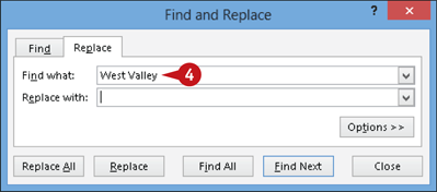
Excel displays the Replace tab of the Find and Replace dialog box.
Type the information for which you want to search here.

Type the information that you want Excel to use to replace the information you typed in Step 4.
Click Find Next.

B Excel finds the first occurrence of the data.
Click Replace.
Excel replaces the information in the cell.
C Excel finds the next occurrence automatically.
 Repeat Step 7 until you replace all appropriate occurrences.
Note: You can click Replace All if you do not want to review each occurrence before Excel replaces it.
Excel displays a message when it cannot find any more occurrences.
 Click OK and then click Close in the Find and Replace dialog box.
Create a Table
You can create a table from any rectangular range of related data in a worksheet. A table is a collection of related information. Table rows — called records — contain information about one element, and table columns divide the element into fields. In a table containing name and address information, a record would contain all the information about one person, and all first names, last names, addresses, and so on would appear in separate columns.
When you create a table, Excel identifies the information in the range as a table and simultaneously formats the table and adds AutoFilter arrows to each column.
Create a Table

Set up a range in a worksheet that contains similar information for each row.
Click anywhere in the range.

Click the Insert tab.
Click Table.

The Create Table dialog box appears, displaying a suggested range for the table.
A You can deselect this option ( changes to ) if labels for each column do not appear in Row 1.
B You can click  to select a new range for the table boundaries by dragging in the worksheet.
Click OK.
Excel creates a table and applies a table style to it.

C The Table Tools Design tab appears on the Ribbon.
D appears in each column title.
E Excel assigns the table a generic name.
simplify it
When should I use a table?
If you need to identify common information, such as the largest value in a range, or you need to select records that match a criterion, use a table. Tables make ranges easy to navigate. When you press  with the cell pointer in a table, the cell pointer stays in the table, moving directly to the next cell and to the next table row when you tab from the last column. When you scroll down a table so that the header row disappears, Excel replaces the column letters with the labels that appear in the header row.
Filter or Sort Table Information
When you create a table, Excel automatically adds AutoFilter arrows to each column; you can use these arrows to quickly and easily filter and sort the information in the table.
When you filter a table, you display only those rows that meet conditions you specify, and you specify those conditions by making selections from the AutoFilter lists. You can also use the AutoFilter arrows to sort information in a variety of ways. Excel recognizes the type of data stored in table columns and offers you sorting choices that are appropriate for the type of data.
Filter or Sort Table Information
Filter a Table
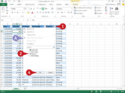
Click next to the column heading you want to use for filtering.
A Excel displays a list of possible filters for the selected column.
Select a filter choice ( changes to or changes to ).
Repeat Step 2 until you have selected all of the filters you want to use.
Click OK.

B Excel displays only the data meeting the criteria you selected in Step 2.
C The AutoFilter changes to  to indicate the data in the column is filtered.
Sort a Table

Click next to the column heading you want to use for sorting.
D Excel displays a list of possible sort orders.
Click a sort order.
This example sorts from smallest to largest.
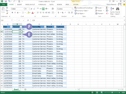
E Excel reorders the information.
F changes to  to indicate the data in the column is sorted.
simplify it
How does the Sort by Color option work?
If you apply font colors, cell colors, or both to some cells in the table, you can then sort the table information by the colors you assigned. You can manually assign colors or you can assign colors using Conditional Formatting; see Chapter 9 for details on using Conditional Formatting.
I do not see the AutoFilter down arrow beside my table headings. What should I do?
Click the Data tab and then click the Filter button. This button toggles on and off the appearance of the AutoFilter in a table.
Analyze Data Quickly
You can easily analyze data in a variety of ways using the Quick Analysis button. You can apply various types of conditional formatting, create different types of charts, or add miniature graphs called sparklines (see Chapter 12 for details on sparkline charts). You can also sum, average, and count occurrences of data as well as calculate percentage of total and running total values. In addition, you can apply a table style and create a variety of different PivotTables.
The choices displayed in each analysis category are not always the same; the ones you see depend on the type of data you select.
Analyze Data Quickly
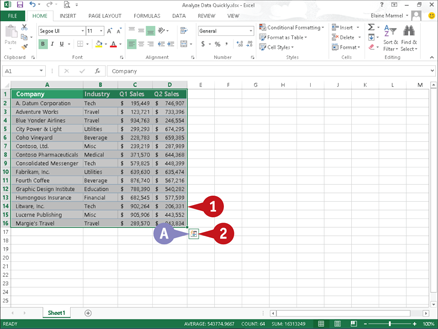
Select a range of data to analyze.
A The Quick Analysis button ( ) appears.
Click .

Quick Analysis categories appear.
Click each category heading to view the options for that category.
Point the mouse at a choice under a category.
B A preview of that analysis choice appears.
Note: For an explanation of the Quick Analysis choices, see the next section, “Understanding Data Analysis Choices.”
When you find the analysis choice you want to use, click it and Excel creates it.
Understanding Data Analysis Choices
The Quick Analysis button offers a variety of ways to analyze selected data. This section provides an overview of the analysis categories and the choices offered in each category.
Formatting
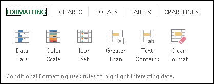
Use formatting to highlight parts of your data. With formatting, you can add data bars, color scales, and icon sets. You can also highlight values that exceed a specified number and cells that contain specified text.
Charts

Pictures often get your point across better than raw numbers. You can quickly chart your data; Excel recommends different chart types based on the data you select. If you do not see the chart type you want to create, you can click More Charts.
Totals
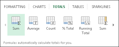
Using the options in the Totals category, you can easily calculate sums — of both rows and columns — as well as averages, percentage of total, and the number of occurrences of the values in the range. You can also insert a running total that grows as you add items to your data.
Tables

Using the choices under the Tables category, you can convert a range to a table, making it easy to filter and sort your data. You can also quickly and easily create a variety of PivotTables — Excel suggests PivotTables you might want to consider and then creates any you might choose.
Sparklines
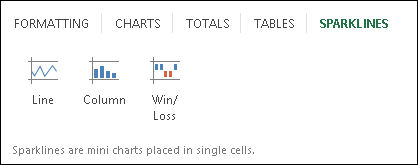
Sparklines are tiny charts that you can display beside your data that provide trend information for selected data. See Chapter 12 for more information on sparkline charts.
Track and Review Worksheet Changes
If you share your Excel workbooks with others, you can use the program’s Track Changes feature to help you keep track of the edits others have made, including formatting changes and data additions or deletions. When you enable tracking, Excel automatically shares the workbook. As you set up tracking options, you can identify the changes you want Excel to highlight. When tracking changes, Excel adds comments that summarize the type of change made. Excel also displays a dark-blue box around a cell that has been changed, and a small blue triangle appears in the upper-left corner of the changed cell.
Track and Review Worksheet Changes
Turn On Tracking

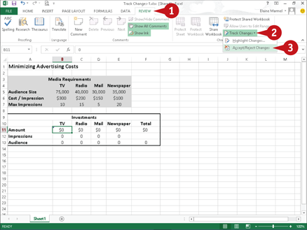
Click the Review tab.
Click Track Changes.
Click Highlight Changes.

The Highlight Changes dialog box appears.
Select Track changes while editing ( changes to ).
Excel automatically shares the workbook file if you have not previously shared it.
A You can select options to determine when, by whom, or where Excel tracks changes.
B You can leave this option selected to display changes on-screen.
Click OK.

Excel prompts you to save the workbook.
Type a filename.
Click Save.

Excel shares the workbook and begins tracking changes to it.
Edit your worksheet.
C Excel places a dark-blue box around changed cells, and a small blue triangle appears in the upper-left corner of the changed cell.
D To view details about a change, position the mouse pointer over the highlighted cell.
Reviewing edits made to a workbook is simple. When you review a workbook in which Excel tracked changes, you can specify whose edits you want to review and what types of edits you want to see. Excel automatically locates and highlights the first edit in a worksheet and gives you the option to accept or reject the edit. After you make your selection, Excel automatically locates and selects the next edit, and so on. You can accept or reject edits one at a time or accept or reject all edits in the worksheet at once.
When you finish reviewing, you can turn off tracking.
Review Changes
Click the Review tab.
Click Track Changes.
Click Accept/Reject Changes.

Excel prompts you to save the file.
Click OK.
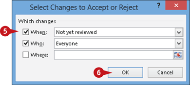
The Select Changes to Accept or Reject dialog box appears.
Click options for which changes you want to view.
Click OK.
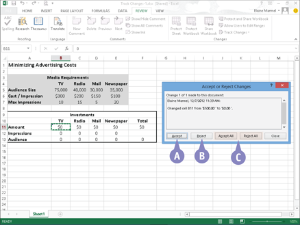
The Accept or Reject Changes dialog box appears.
Specify an action for each edit:
A You can click Accept to add the change to the final worksheet.
B You can click Reject to reject the change.
C You can click one of these options to accept or reject all of the changes at the same time.
simplify it
How can I stop tracking changes?

To turn off Track Changes, follow these steps:
Click the Review tab.
Click the Track Changes button.
Click Highlight Changes.
In the Highlight Changes dialog box that appears, deselect Track changes while editing ( changes to ).
Click OK. A message appears, explaining the consequences of no longer sharing the workbook; click OK.
Insert a Comment
You can add comments to your worksheets. You might add a comment to make a note to yourself about a particular cell’s contents, or you might include a comment as a note for other users to see. For example, if you share your workbooks with other users, you can use comments to leave feedback about the data without typing directly in the worksheet.
When you add a comment to a cell, Excel displays a small red triangle in the upper-right corner of the cell until you choose to view it. Comments you add are identified with your username.
Insert a Comment
Add a Comment

Click the cell to which you want to add a comment.
Click the Review tab on the Ribbon.
Click the New Comment button.
You can also right-click the cell and choose Insert Comment.

A comment balloon appears.
Type your comment text.

Click anywhere outside the comment balloon to deselect the comment.
A Cells that contain comments display a tiny red triangle in the corner.
View a Comment

Position the mouse pointer over the cell.
B The comment balloon appears, displaying the comment.