Chapter 11: Working with Formulas and Functions
Understanding Formulas
You can use formulas, which you build using mathematical operators, values, and cell references, to perform all kinds of calculations on your Excel data. For example, you can add the contents of a column of monthly sales totals to determine the cumulative sales total.
If you are new to writing formulas, this section explains the basics of building your own formulas in Excel. You learn about the correct way to structure formulas in Excel, how to reference cell data in your formulas, which mathematical operators are available for your use, and more.
Formula Structure

Ordinarily, when you write a mathematical formula, you write the values and the operators, followed by an equal sign, such as 2+2=. In Excel, formula structure works a bit differently. All Excel formulas begin with an equal sign (=), such as =2+2. The equal sign tells Excel to recognize any subsequent data as a formula rather than as a regular cell entry.
Reference a Cell

Every cell in a worksheet has a unique address, composed of the cell’s column letter and row number, and that address appears in the Name box to the left of the Formula bar. Cell B3, for example, identifies the third cell down in column B. Although you can enter specific values in your Excel formulas, you can make your formulas more versatile if you include — that is, reference — a cell address instead of the value in that cell. Then, if the data in the cell changes but the formula remains the same, Excel automatically updates the result of the formula.
Cell Ranges

A group of related cells in a worksheet is called a range. Excel identifies a range by the cells in the upper-left and lower-right corners of the range, separated by a colon. For example, range A1:B3 includes cells A1, A2, A3, B1, B2, and B3. You can also assign names to ranges to make it easier to identify their contents. Range names must start with a letter, underscore, or backslash, and can include uppercase and lowercase letters. Spaces are not allowed.
Mathematical Operators
You use mathematical operators in Excel to build formulas. Basic operators include the following:
|
Operator |
Operation |
|
+ |
Addition |
|
- |
Subtraction |
|
* |
Multiplication |
|
/ |
Division |
|
% |
Percentage |
|
^ |
Exponentiation |
|
= |
Equal to |
|
< |
Less than |
|
<= |
Less than or equal to |
|
> |
Greater than |
|
>= |
Greater than or equal to |
|
<> |
Not equal to |
Operator Precedence
Excel performs operations from left to right, but gives some operators precedence over others, following the rules you learned in high school math:
|
Order |
Operation |
|
First |
All operations enclosed in parentheses |
|
Second |
Exponential operations |
|
Third |
Multiplication and division |
|
Fourth |
Addition and subtraction |
When you are creating equations, the order of operations determines the results. For example, suppose you want to determine the average of values in cells A2, B2, and C2. If you enter the equation =A2+B2+C2/3, Excel first divides the value in cell C2 by 3, and then adds that result to A2+B2 — producing the wrong answer. The correct way to write the formula is =(A2+B2+C2)/3. By enclosing the values in parentheses, you are telling Excel to perform the addition operations in the parentheses before dividing the sum by 3.
Reference Operators
You can use Excel’s reference operators to control how a formula groups cells and ranges to perform calculations. For example, if your formula needs to include the cell range D2:D10 and cell E10, you can instruct Excel to evaluate all the data contained in these cells using a reference operator. Your formula might look like this: =SUM(D2:D10,E10).
|
Operator |
Example |
Operation |
|
: |
=SUM(D3:E12) |
Range operator. Evaluates the reference as a single reference, including all of the cells in the range from both corners of the reference. |
|
, |
=SUM(D3:E12,F3) |
Union operator. Evaluates the two references as a single reference. |
|
[space] |
=SUM(D3:D20 D10:E15) |
Intersect operator. Evaluates the cells common to both references. |
|
[space] |
=SUM(Totals Sales) |
Intersect operator. Evaluates the intersecting cell or cells of the column labeled Totals and the row labeled Sales. |
Create a Formula
You can write a formula to perform a calculation on data in your worksheet. In Excel, all formulas begin with an equal sign (=) and contain the values or cell references to the cells that contain the relevant values. For example, the formula for adding the contents of cells C3 and C4 together is =C3+C4. You create formulas in the Formula bar; formula results appear in the cell to which you assign a formula.
Note that, in addition to referring to cells in the current worksheet, you can also build formulas that refer to cells in other worksheets.
Create a Formula

 Click the cell where you want to place a formula.
 Type =.
A Excel displays the formula in the Formula bar and in the active cell.
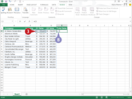
 Click the first cell that you want to include in the formula.
B Excel inserts the cell reference into the formula.
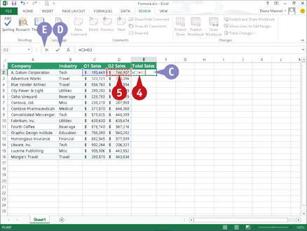
 Type an operator for the formula.
 Click the next cell that you want to include in the formula.
C Excel inserts the cell reference into the formula.
 Repeat Steps 4 and 5 until all the necessary cells and operators have been added.
 Press
Press  .
.
D You can also click Enter ( ) on the Formula bar to accept the formula.
E You can click Cancel ( ) to cancel the formula.

F The result of the formula appears in the cell.
G The formula appears in the Formula bar; you can view it by clicking the cell containing the formula.
Note: If you change a value in a cell referenced in your formula, Excel automatically updates the formula result to reflect the change.
simplify it
How do I edit a formula?
To edit a formula, click in the cell containing the formula and make any corrections in the Formula bar. Alternatively, double-click in the cell to make edits to the formula from within the cell. When finished, press or click Enter () on the Formula bar.
How do I reference cells in other worksheets?
To reference a cell in another worksheet, specify the worksheet name followed by an exclamation mark and then the cell address (for example, Sheet2!D12 or Sales!D12). If the worksheet name includes spaces, enclose the sheet name in single quote marks, as in ‘Sales Totals’!D12.
Apply Absolute and Relative Cell References
By default, Excel uses relative cell referencing. If you copy a formula containing a relative cell reference to a new location, Excel adjusts the cell addresses in that formula to refer to the cells at the formula’s new location. For example, if you enter, in cell B8, the formula =B5+B6 and then you copy that formula to cell C8, Excel adjusts the formula to =C5+C6.
When a formula must always refer to the value in a particular cell, use an absolute cell reference. Absolute references are preceded with dollar signs. If your formula must always refer to the value in cell D2, enter $D$2 in the formula.
Apply Absolute and Relative Cell References
Copy Relative References

Enter the formula.
Click the cell containing the formula you want to copy.
A In the Formula bar, the formula appears with a relative cell reference.
Click the Home tab.
Click Copy ( ).
).

Select the cells where you want the formula to appear.
Click Paste.
B Excel copies the formula to the selected cells.
C The adjusted formula appears in the Formula bar and in the selected cells.
Copy Absolute References

Enter the formula, including dollar signs ($) for absolute addresses as needed.
Click the cell containing the formula you want to copy.
D In the Formula bar, the formula appears with an absolute cell reference.
Click the Home tab.
Click Copy ().

Select the cells where you want the formula to appear.
Click Paste.
E Excel copies the formula to the selected cells.
F The formula in the selected cells adjusts only relative cell references; absolute cell references remain unchanged.
Understanding Functions
If you are looking for a speedier way to enter formulas, you can use any one of a wide variety of functions. Functions are ready-made formulas that perform a series of operations on a specified range of values. Excel offers more than 300 functions, grouped into 13 categories, that you can use to perform various types of calculations.
Functions use arguments to identify the cells that contain the data you want to use in your calculations. Functions can refer to individual cells or to ranges of cells. This section explains the basics of working with functions.
Function Elements
All functions must start with an equal sign (=). Functions are distinct in that each one has a name. For example, the function that sums data is called SUM, and the function for averaging values is called AVERAGE. You can create functions by typing them directly into your worksheet cells or the Formula bar; alternatively, you can use the Insert Function dialog box to select and apply functions to your data.
Construct an Argument

Functions use arguments to indicate which cells contain the values you want to calculate. Arguments are enclosed in parentheses. When applying a function to individual cells in a worksheet, you can use a comma to separate the cell addresses, as in =SUM(A5,C5,F5). When applying a function to a range of cells, you can use a colon to designate the first and last cells in the range, as in =SUM(B4:G4). If your range has a name, you can insert the name, as in =SUM(Sales).
Types of Functions
Excel groups functions into 13 categories, not including functions installed with Excel add-in programs:
|
Category |
Description |
|
Financial |
Includes functions for calculating loans, principal, interest, yield, and depreciation. |
|
Date & Time |
Includes functions for calculating dates, times, and minutes. |
|
Math & Trig |
Includes a wide variety of functions for calculations of all types. |
|
Statistical |
Includes functions for calculating averages, probabilities, rankings, trends, and more. |
|
Lookup & Reference |
Includes functions that enable you to locate references or specific values in your worksheets. |
|
Database |
Includes functions for counting, adding, and filtering database items. |
|
Text |
Includes text-based functions to search and replace data and other text tasks. |
|
Logical |
Includes functions for logical conjectures, such as if-then statements. |
|
Information |
Includes functions for testing your data. |
|
Engineering |
Offers many kinds of functions for engineering calculations. |
|
Cube |
Enables Excel to fetch data from SQL Server Analysis Services, such as members, sets, aggregated values, properties, and KPIs. |
|
Compatibility |
Use these functions to keep your workbook compatible with earlier versions of Excel. |
|
Web |
Use these functions when you work with web pages, services, or XML content. |
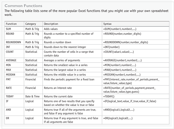
Common Functions
Apply a Function
You can use functions to speed up your Excel calculations. Functions are ready-made formulas that perform a series of operations on a specified range of values.
You use the Insert Function dialog box, which acts like a wizard, to look for a particular function from among Excel’s 300-plus available functions and to guide you through successfully entering the function. After you select your function, the Function Arguments dialog box opens to help you build the formula by describing the arguments you need for the function you chose. Functions use arguments to indicate that the cells contain the data you want to use in your calculation.
Apply a Function
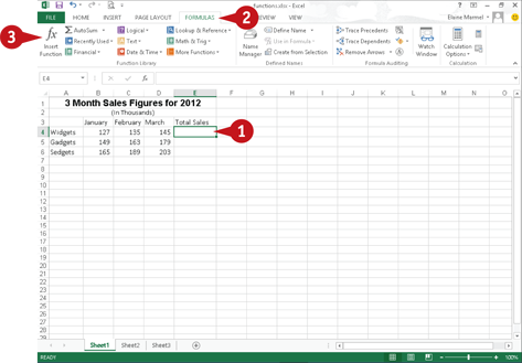
Click the cell in which you want to store the function.
Click the Formulas tab.
Click the Insert Function button.

A Excel inserts an equal sign to indicate that a formula follows.
Excel displays the Insert Function dialog box.
Type a description of the function you need here.
Click Go.
B A list of suggested functions appears.
Click the function that you want to apply.
C A description of the selected function appears here.
Click OK.

The Function Arguments dialog box appears.
 Select the cells for each argument required by the function.
In the worksheet, Excel adds the cells as the argument to the function.
D Additional information about the function appears here.
 When you finish constructing the arguments, click OK.

E Excel displays the function results in the cell.
F The function appears in the Formula bar.
Total Cells with AutoSum
One of the most popular Excel functions is the AutoSum function. AutoSum automatically totals the contents of cells. For example, you can quickly total a column of sales figures. One way to use AutoSum is to select a cell and let the function guess which surrounding cells you want to total. Alternatively, you can specify exactly which cells to sum.
In addition to using AutoSum to total cells, you can simply select a series of cells in your worksheet; Excel displays the total of the cells’ contents in the status bar, along with the number of cells you selected and an average of their values.
Total Cells with AutoSum
Using AutoSum to Total Cells

Click the cell in which you want to store a total.
Click the Formulas tab.
Click the AutoSum button.
A If you click the AutoSum  , you can select other common functions, such as Average or Max.
You can also click the AutoSum button ( ) on the Home tab.

B AutoSum generates a formula to total the adjacent cells.
Press or click Enter ().

C Excel displays the result in the cell.
D You can click the cell to see the function in the Formula bar.
Total Cells without Applying a Function

Click a group of cells whose values you want to total.
Note: To sum noncontiguous cells, press and hold  while clicking the cells.
E Excel adds the contents of the cells, displaying the sum in the status bar along the bottom of the program window.
F Excel also counts the number of cells you have selected.
G Excel also displays an average of the values in the selected cells.
simplify it
Can I select a different range of cells to sum?
Yes. AutoSum takes its best guess when determining which cells to total. If it guesses wrong, simply click the cells you want to add together before pressing or clicking Enter ().
Why do I see pound signs (#) in a cell that contains a SUM function?
Excel displays pound signs in any cell — not just cells containing formulas or functions — when the cell’s column is not wide enough to display the contents of the cell, including the cell’s formatting. Widen the column to correct the problem; see Chapter 9 for details.
Audit a Worksheet for Errors
On occasion, you may see an error message, such as #DIV/0! or #NAME?, in your Excel worksheet. If you do, you should double-check your formula references to ensure that you included the correct cells. Locating the source of an error can be difficult, however, especially in larger worksheets. Fortunately, if an error occurs in your worksheet, you can use Excel’s Formula Auditing tools — namely, Error Checking and Trace Error — to examine and correct formula errors. For more information on types of errors and how to resolve them, see the table in the tip.
Audit a Worksheet for Errors
Apply Error Checking

Click the Formulas tab.
Click the Error Checking button ( ).
).
A Excel displays the Error Checking dialog box and highlights the first cell containing an error.
To fix the error, click Edit in Formula Bar.
B To find help with an error, you can click here to open the help files.
C To ignore the error, you can click Ignore Error.
D You can click Previous and Next to scroll through all of the errors on the worksheet.
Make edits to the cell references in the Formula bar or in the worksheet.

Click Resume.
When the error check is complete, a message box appears.
Click OK.
Trace Errors
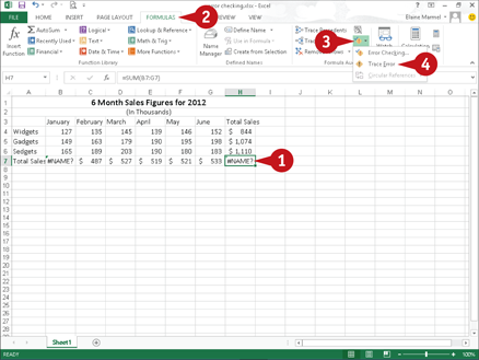
Click the cell containing the formula or function error that you want to trace.
Click the Formulas tab.
Click the Error Checking .
Click Trace Error.
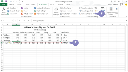
E Excel displays trace lines from the current cell to any cells referenced in the formula.
You can make changes to the cell contents or changes to the formula to correct the error.
F You can click Remove Arrows to turn off the trace lines.