Therefore, the code for calculating the histogram for a full grayscale image (without a mask) is as follows:
image = cv2.imread('lenna.png')
gray_image = cv2.cvtColor(image, cv2.COLOR_BGR2GRAY)
hist = cv2.calcHist([gray_image], [0], None, [256], [0, 256])
In this case, hist is a (256, 1) array. Each value (bin) of the array corresponds to the number of pixels (frequency) with the corresponding tone value.
To plot histograms with Matplotlib, you can use plt.plot(), providing the histogram and the color to show the histogram (example, color='m'). The following color abbreviations are supported—'b'—blue, 'g'—green, ‘r’—red, 'c'—cyan, 'm'—magenta, 'y'—yellow, 'k'—black, and 'w'—white. The full code for this example can be seen in the grayscale_histogram.py script.
We commented in the introduction that histograms can be used to reveal or detect image acquisition issues. The following example will show you how to detect image brightness issues. The brightness of a grayscale image can be defined as the average intensity of all the pixels of the image given by the following formulation:

Here, I(x, y) is the tone value for a specific pixel of the image.
Therefore, if the average tone of an image is high (for example, 220), this means that most pixels of the image will be very close to the white color. On the contrary, if the average tone on an image is low (for example, 30) this means that most pixels of the image will be very close to the black color.
In the aforementioned script, grayscale_histogram.py, we will see how to change the brightness of an image and how the histogram changes.
In this script, which has already been introduced in order to show how a histogram can be calculated and shown for a grayscale image, we also performed some basic math on the grayscale-loaded image. Specifically, we have performed both image addition and subtraction in order to add/subtract a specific quantity to or from the gray level intensity of every pixel of the image. This can be performed with the cv2.add() and cv2.subtract() functions.
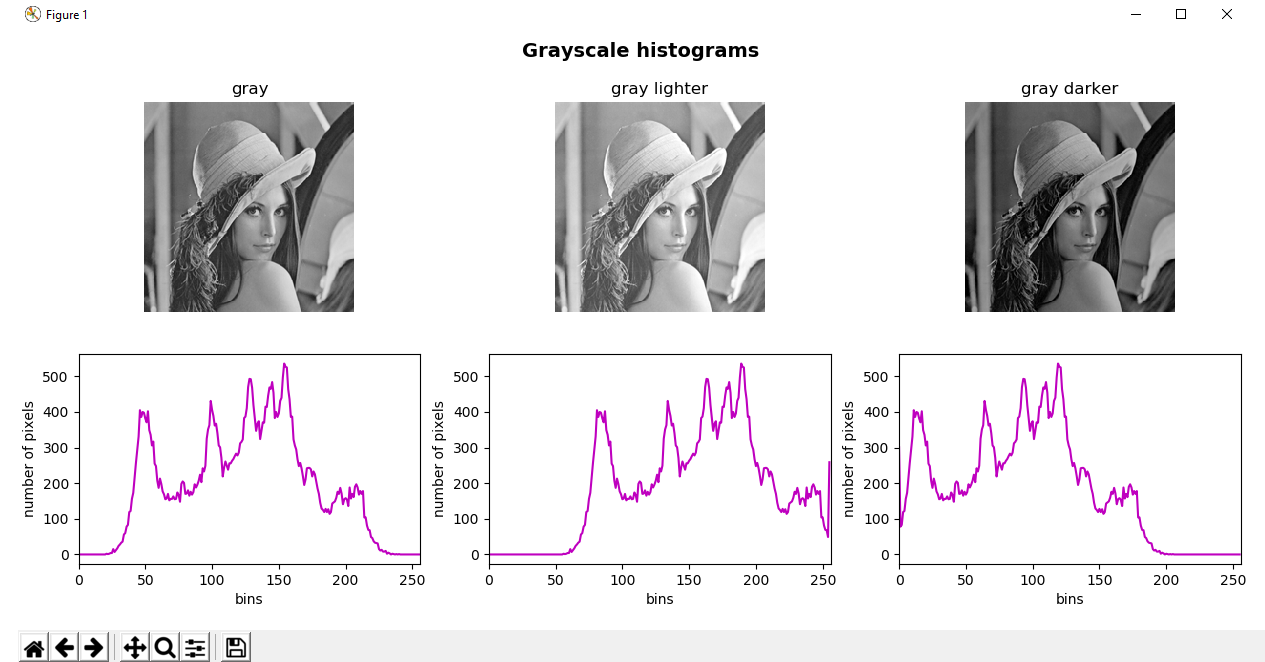
In this way, the average brightness level of the image can be shifted. This can be seen in the next screenshot, corresponding to the output of the script:

In this specific case, we have added/subtracted 35 to/from every pixel of the original image, and then calculated the histogram for the resulting images:
# Add 35 to every pixel on the grayscale image (the result will look lighter) and calculate histogram
M = np.ones(gray_image.shape, dtype="uint8") * 35
added_image = cv2.add(gray_image, M)
hist_added_image = cv2.calcHist([added_image], [0], None, [256], [0, 256])

# Subtract 35 from every pixel (the result will look darker) and calculate histogram
subtracted_image = cv2.subtract(gray_image, M)
hist_subtracted_image = cv2.calcHist([subtracted_image], [0], None, [256], [0, 256])
As you can see, the central grayscale image corresponds to the image where 35 is added to every pixel of the original image, resulting in a lighter image. In this image, the histogram appears shifted to the right, in the sense that there are no pixels with intensities in the range [0-35]. On the contrary, the grayscale image on the right corresponds to the image where 35 is subtracted from every pixel of the original image, resulting in a darker image. The histogram appears shifted to the left, in the sense that there are no pixels with intensities in the range [220-255].