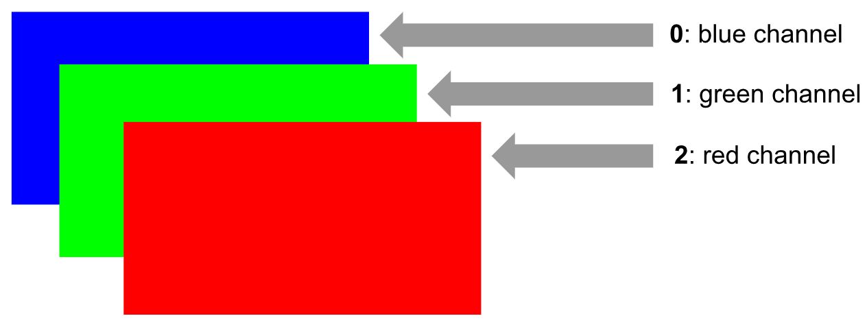
We already mentioned that OpenCV uses the BGR color format instead of the RGB one. This can be seen in the following diagram, where you can see the order of the three channels:
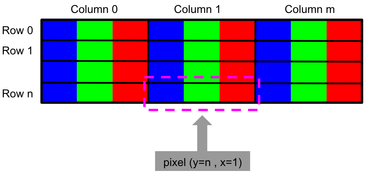
The pixel structure of a BGR image can be seen in the following diagram. In particular, we have detailed how to access pixel (y=n, x=1) for clarification purposes:
Initial developers at OpenCV chose the BGR color format (instead of the RGB one) because at the time, the BGR color format was very popular among software providers and camera manufacturers. For example, in Windows, when specifying a color value using COLORREF, they used the BGR format, 0x00bbggrr (https://docs.microsoft.com/es-es/windows/desktop/gdi/colorref). In summary, BGR was chosen for historical reasons.
Additionally, other Python packages use the RGB color format. Therefore, we need to know how to convert an image from one format into the other. For example, Matplotlib uses the RGB color format. Matplotlib (https://matplotlib.org/) is the most popular 2D Python plotting library and offers you a wide variety of plotting methods. You can interact with the plotted images (for example, zoom into images and save them). Matplotlib can be used both in Python scripts or in the Jupyter Notebook. You can check out the Matplotlib documentation for further details (https://matplotlib.org/contents.html).
Therefore, a good choice for your projects is to show the images using the Matplotlib package instead of the functionality offered by OpenCV. Now we are going to see now how we can deal with the different color formats in the two libraries.
First of all, we load the image using the cv2.imread() function:
# Load image using cv2.imread:
img_OpenCV = cv2.imread('logo.png')
The image is stored in the img_OpenCV variable because the cv2.imread() function loads the image in BGR order. Then, we split the loaded image into its three channels, (b, g, r), using the cv2.split() function. The parameter of this function is the image we want to split:
# Split the loaded image into its three channels (b, g, r):
b, g, r = cv2.split(img_OpenCV)
The next step is to merge the channels again (in order to build a new image based on the information provided by the channels) but in a different order. We change the order of the b and r channels in order to follow the RGB format, that is, the one we need for Matplotlib:
# Merge again the three channels but in the RGB format:
img_matplotlib = cv2.merge([r, g, b])
At this point, we have two images (img_OpenCV and img_matplotlib), which are going to be plotted with both OpenCV and Matplotlib so that we can see the results. First of all, we will show these two images with Matplotlib.
To show the two images with Matplotlib in the same window, we will use subplot, which places multiple images within the same window. You have three parameters to use within subplot, for example subplot(m,n,p). In this case, subplot handles plots in a m x n grid, where m establishes the number of rows, n establishes the number of columns, and p establishes where you want to place your plot in the grid. To show the images with Matplotlib, we will use imshow.
In this case, as we are showing two images horizontally, m = 1 and n = 2. We will be using p = 1 for the first subfigure (img_OpenCV) and p = 2 for the second subfigure ( img_matplotlib ):
# Show both images (img_OpenCV and img_matplotlib) using matplotlib
# This will show the image in wrong color:
plt.subplot(121)
plt.imshow(img_OpenCV)
# This will show the image in true color:
plt.subplot(122)
plt.imshow(img_matplotlib)
plt.show()
Therefore, the output you will get should be very similar to the output that's shown in the following diagram:
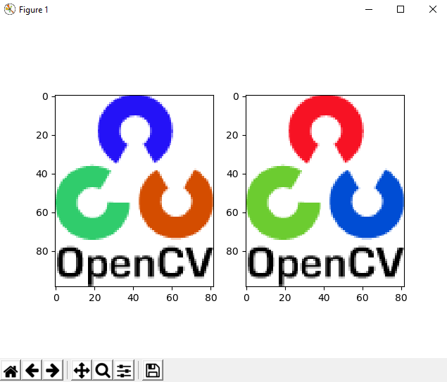
As you can see, the first subfigure shows the image in the wrong color (BGR order), while the second subfigure shows the image in true color (RGB order). In the same way, we will show the two images using cv2.imshow():
# Show both images (img_OpenCV and img_matplotlib) using cv2.imshow()
# This will show the image in true color:
cv2.imshow('bgr image', img_OpenCV)
# This will show the image in wrong color:
cv2.imshow('rgb image', img_matplotlib)
cv2.waitKey(0)
cv2.destroyAllWindows()
The following screenshot shows what you will get from executing the previous code:

As expected, the screenshot shows the image in true color, while the second figure shows the image in the wrong color.
Additionally, if we want to show the two images in the same window, we can build a full image that contains the two images, concatenating them horizontally. To do so, we will use NumPy's concatenate() method. The parameters of this method are the two images to concatenate and the axis. In this case, axis = 1 (to stack them horizontally):
# To stack horizontally (img_OpenCV to the left of img_matplotlib):
img_concats = np.concatenate((img_OpenCV, img_matplotlib), axis=1)
# Now, we show the concatenated image:
cv2.imshow('bgr image and rgb image', img_concats)
cv2.waitKey(0)
cv2.destroyAllWindows()
Check out the following screenshot to see the concatenated image:

One consideration to take into account is that cv2.split() is a time-consuming operation. Depending on your needs, consider using NumPy indexing. For example, if you want to get one channel of the image, instead of using cv2.split() to get the desired channel, you can use NumPy indexing. See the following example to get the channels using NumPy indexing:
# Using numpy capabilities to get the channels and to build the RGB image
# Get the three channels (instead of using cv2.split):
B = img_OpenCV[:, :, 0]
G = img_OpenCV[:, :, 1]
R = img_OpenCV[:, :, 2]
Another consideration is that you can use NumPy for converting the image from BGR into RGB in a single instruction:
# Transform the image BGR to RGB using Numpy capabilities:
img_matplotlib = img_OpenCV[:, :, ::-1]
To summarize everything in this chapter, we have created two Jupiter Notebooks. In these notebooks, you can play with all of the concepts that have been introduced so far:
- Getting-And-Setting-BGR.ipynb
- Getting-And-Setting-GrayScale.ipynb
Taking advantage of the benefits notebook (and all of the information included in this chapter), no additional information is needed to play with them. So, go ahead and try it for yourself. Remember (see Chapter 1, Setting Up OpenCV) that to run the notebook, you need to run the following command at the Terminal (Mac/Linux) or Command Prompt (Windows):
$ jupyter notebook
This command will print information in connection with the notebook server, including the URL of the web application (by default, this URL is http://localhost:8888). Additionally, this command will also open your web browser pointing to this URL:
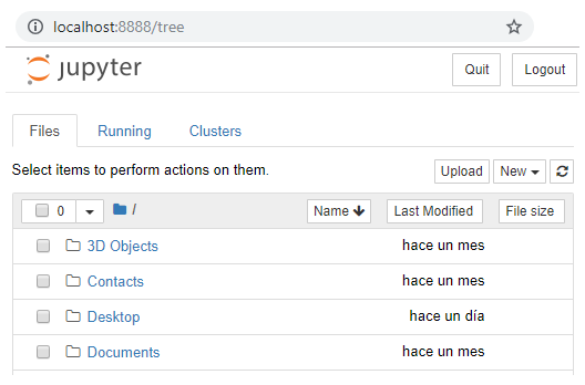
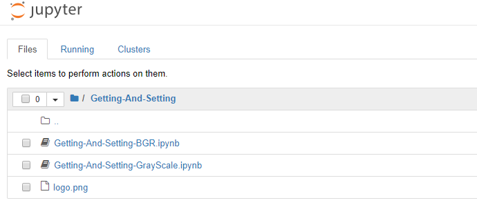
At this point, you are able to upload the Getting-And-Setting-BGR.ipynb and Getting-And-Setting-GrayScale.ipynb files by clicking on the Upload button (see the previous screenshot). These files use the logo.png image. Therefore, you should upload this image in the same way. After loading these three files, you should see these files loaded:
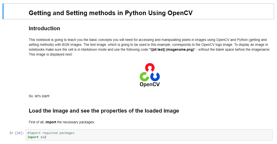
At this point, you can open these notebooks by clicking on them. You should see the content of the notebook, which is shown in the following screenshot:
Finally, you can start executing the loaded notebook document. You can execute the notebook step by step (one cell a time) by pressing Shift + Enter. Additionally, you can execute the whole notebook in a single step by clicking on the Cell | Run All menu. Moreover, you can also restart the kernel (the computational engine) by clicking on the Kernel | Restart menu.