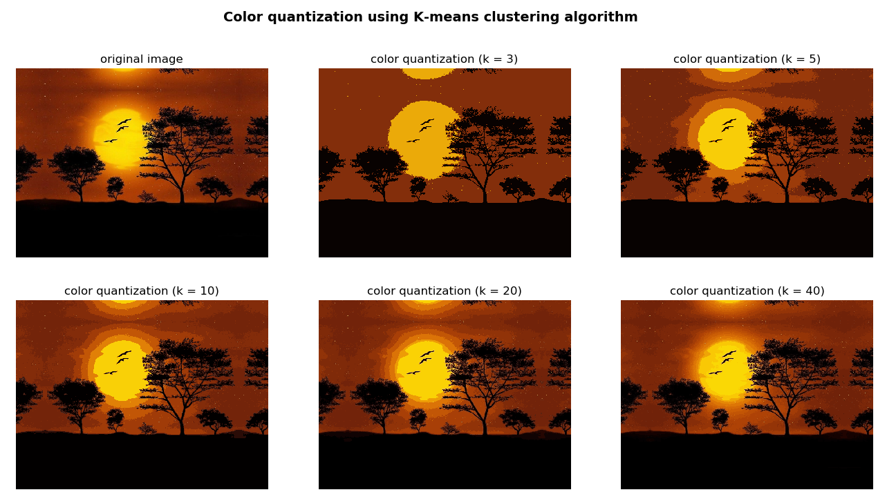
In this subsection, we will apply the k-means clustering algorithm to the problem of color quantization, which can be defined as the process of reducing the number of colors in an image. Color quantization is a critical point for displaying images on certain devices that can only display a limited number of colors (commonly due to memory restrictions). Therefore, a trade-off between the similarity and the reduction in the number of colors is usually necessary. This trade-off is established by setting the K parameter properly, as we will see in the next examples.
In the k_means_color_quantization.py script, we perform the k-means clustering algorithm to perform color quantization. In this case, each element of the data is composed of 3 features, which correspond to the B, G, and R values for each of the pixels of the image. Therefore, the key step is to transform the image into data this way:
data = np.float32(image).reshape((-1, 3))
Here, image is the image we previously loaded.
In this script, we performed the clustering procedure using several values of K (3, 5, 10, 20, and 40) in order to see how the resulting image changes. For example, if we want the resulting image with only 3 colors (K = 3), we must perform the following:
- Load the BGR image:
img = cv2.imread('landscape_1.jpg')
- Perform color quantization using the color_quantization() function:
color_3 = color_quantization(img, 3)
- Show both images in order to see the results. The color_quantization() function performs the color quantization procedure:
def color_quantization(image, k):
    """Performs color quantization using K-means clustering algorithm"""

    # Transform image into 'data':
    data = np.float32(image).reshape((-1, 3))
    # print(data.shape)

    # Define the algorithm termination criteria (maximum number of iterations and/or required accuracy):
    # In this case the maximum number of iterations is set to 20 and epsilon = 1.0
    criteria = (cv2.TERM_CRITERIA_EPS + cv2.TERM_CRITERIA_MAX_ITER, 20, 1.0)

    # Apply K-means clustering algorithm:
    ret, label, center = cv2.kmeans(data, k, None, criteria, 10, cv2.KMEANS_RANDOM_CENTERS)

    # At this point we can make the image with k colors
    # Convert center to uint8:
    center = np.uint8(center)
    # Replace pixel values with their center value:
    result = center[label.flatten()]
    result = result.reshape(img.shape)
    return result
In the previous function, the key point is to make use of cv2.kmeans() method. Finally, we can build the image with k colors replacing each pixel value with their corresponding center value. The output of this script can be seen in the next screenshot:

The previous script can be extended to include an interesting functionality, which shows the number of pixels assigned to each center value. This can be seen in the k_means_color_quantization_distribution.py script.
The color_quantization() function has been modified to include this functionality:
def color_quantization(image, k):
    """Performs color quantization using K-means clustering algorithm"""

    # Transform image into 'data':
    data = np.float32(image).reshape((-1, 3))
    # print(data.shape)

    # Define the algorithm termination criteria (the maximum number of iterations and/or the desired accuracy):
    # In this case the maximum number of iterations is set to 20 and epsilon = 1.0
    criteria = (cv2.TERM_CRITERIA_EPS + cv2.TERM_CRITERIA_MAX_ITER, 20, 1.0)

    # Apply K-means clustering algorithm:
    ret, label, center = cv2.kmeans(data, k, None, criteria, 10, cv2.KMEANS_RANDOM_CENTERS)

    # At this point we can make the image with k colors
    # Convert center to uint8:
    center = np.uint8(center)
    # Replace pixel values with their center value:
    result = center[label.flatten()]
    result = result.reshape(img.shape)

    # Build the 'color_distribution' legend.
    # We will use the number of pixels assigned to each center value:
    counter = collections.Counter(label.flatten())
    print(counter)

    # Calculate the total number of pixels of the input image:
    total = img.shape[0] * img.shape[1]

    # Assign width and height to the color_distribution image:
    desired_width = img.shape[1]
    # The difference between 'desired_height' and 'desired_height_colors'
    # will be the separation between the images
    desired_height = 70
    desired_height_colors = 50

    # Initialize the color_distribution image:
    color_distribution = np.ones((desired_height, desired_width, 3), dtype="uint8") * 255
    # Initialize start:
    start = 0

    for key, value in counter.items():
        # Calculate the normalized value:
        value_normalized = value / total * desired_width

        # Move end to the right position:
        end = start + value_normalized

        # Draw rectangle corresponding to the current color:
        cv2.rectangle(color_distribution, (int(start), 0), (int(end), desired_height_colors), center[key].tolist(), -1)
        # Update start:
        start = end

    return np.vstack((color_distribution, result))
As you can see, we make use of collections.Counter() to count the number of pixels assigned to each center value:
counter = collections.Counter(label.flatten())
For example, if K = 3—Counter({0: 175300, 2: 114788, 1: 109912}). Once the color-distribution image has been built, the final step is to concatenate both images:
np.vstack((color_distribution, result))
The output of this script can be seen in the next screenshot:

In the previous screenshot you can see the result of applying color quantization using k-means clustering algorithm varying the parameter k (3, 5, 10, 20, and 40). A bigger value of k means a more realistic image.