Chapter 7
Floaters and Linkers
Learning bond math involves building a set of analytical tools. That is what we've been doing for the most part in the first six chapters—rate conversions, pricing and yield calculations, after-tax cash flows, implied spot and implied forward rates, duration, and convexity. The payoff ultimately comes in analyzing bond portfolios and fixed-income strategies, as we'll see in Chapters 9 and 10. But first we can use the toolkit to look at types of debt securities other than the traditional fixed-rate and zero-coupon bonds we've been working with so far.
Floating-rate notes (floaters or FRNs) remind us that trying to minimize interest rate risk in the bond market is rather like squeezing one end of a balloon to make it smaller. Obviously, the future cash flows on a fixed-rate bond are known in advance (barring default, of course). Therefore, interest rate volatility is realized entirely in the fluctuation of current market value. Floaters aim to minimize price volatility, but at the expense of uncertain future cash flows. Interest payments typically are tied to a money market reference rate—for instance, 3-month LIBOR. By design, the duration of a floater is very low, typically close to zero, for changes in market interest rates regardless of the time to maturity.
Inflation-indexed bonds (or linkers) adjust future coupon and/or principal cash flows for realized inflation. The idea is to maintain real value in terms of the purchasing power of future cash flows. There are two designs: (1) The coupon rate is fixed while the principal changes with the consumer price index (CPI), and (2) the principal is fixed while the coupon rate adjusts for changes in the CPI. I like to call the first type “P-Linkers” because the link is to the principal and the second “C-Linkers” because the link is to the coupon rate. Both designs provide the investor with inflation protection—their inflation durations are zero, or at least close to zero. However, their real rate durations can be quite high, even higher than those for traditional fixed-rate bonds of comparable time to maturity.
A theme, actually a subplot, to this chapter is negative duration. That's an oddity for a debt security that does not contain an embedded option. The idea is that the bond price goes up (or down) when interest rates go up (or down). It's the opposite reaction from the usual inverse relationship between bond price and yield. If you work with or have studied floating-rate notes, ask yourself what type of standard FRN (e.g., one paying 3-month LIBOR plus a fixed margin) might have negative duration—a floater trading at a discount or at a premium? If you know the answer to that, try this: When might an inflation-indexed bond, in particular a C-Linker, have negative inflation duration—when it's trading at a discount or at a premium? If you have no idea, read on.
Floating-Rate Notes in General
Interest payments on a standard floating-rate note adjust from period to period to reflect changes in a money market reference rate. The market for floaters started in the 1970s when interest rates began to rise due to “inflation creep,” as it was called back then. Fixed-income bonds, which were seen to be boring compared to the excitement of the stock market, finally became interesting. Interest in bonds arose because conservative, buy-and-hold investors experienced losses, at least in terms of market value, when yields to maturity went up. Floaters, first issued by commercial banks, were offered to investors as a way of “preserving capital value,” meaning that they transferred interest rate risk from market value to future cash flows.
Consider a 10-year, floating-rate note making quarterly interest payments of 3-month LIBOR plus 0.50%. LIBOR is set at the beginning of each period, and the interest payment is made in arrears at the end of the period. In practice, the rate typically is set two business days prior to the start of the period. While there might be a cap or floor on the interest rate, thereby setting a maximum or minimum payment, we'll deal only with “straight floaters” that have no such embedded options. So, if 3-month LIBOR turns out to be 1.50%, the annual interest rate for the period is 2.00%. The interest payment for the quarter will be about $0.50 per $100 of par value, depending on the number of days in the period. Most FRNs use an actual/360 day count in the U.S.; actual/365 is used in many other markets.
Notice that while the money market reference rate varies, the margin over LIBOR is fixed at 50 basis points. That's the key to understanding the market value volatility (i.e., duration) of the floater. LIBOR, the standard reference rate for U.S. dollar-denominated FRNs, captures macroeconomic factors (e.g., expected inflation, monetary policy, and general business conditions). Students are often surprised that one of the most important interest rates in the U.S. financial market is determined in London, not in New York. Moreover, most of the commercial banks that are surveyed each day by the British Bankers Association to set LIBOR are not even headquartered in the U.S. The margin on the FRN, like the spread over the benchmark yield on a fixed-rate bond, captures microeconomic factors (e.g., credit risk of the issuer, liquidity, and taxation).
As long as this floater's “correct” margin continues to be 50 basis points, meaning no change in credit risk, liquidity, or taxation, the FRN will trade at par value on each coupon payment date. The 10-year floater is then the financial equivalent of rolling over a series of 40 short-term time deposits, each paying 3-month LIBOR + 0.50%. Each time deposit is initially like a 3-month zero-coupon money market security having an annual Macaulay duration of about 0.25.
The usual presentation of the interest rate sensitivity of floaters makes the assumption of repricing at par value on each payment date. That is, the duration equals the time remaining in the coupon period. However, assuming no change in credit risk or liquidity severely limits our analysis. The U.S. Treasury does not issue floating-rate notes. Most floaters have been issued by financial institutions that can and do experience downgrades in their credit ratings (and even upgrades once upon a time), as well as changes in liquidity. Fortunately, we can use some bond math tools to build a simple valuation model for floaters. From that model, we can derive an expression for duration.
A Simple Floater Valuation Model
Remember from Chapter 3 that the reason why a fixed-rate bond trades at a premium or discount is that the coupon rate (what you are promised to receive from the issuer) is more or less than the yield to maturity (what you would need to pay par value). The same idea applies to a floating-rate note—the amount of the premium or discount is the present value of the difference between the fixed margin (the “quoted margin”) and the required margin (which, following market terminology, is called the “discount margin”) in order for the floater to trade at par value. The quoted margin is what you get; the discount margin is what you need.
Consider a floating-rate note that resets its interest rate PER times per year—that is the periodicity of the floater. As of the beginning of the current period (date 0), the floater has Z years to maturity, or a total of  periods. Let R0 denote the reference index rate set for date 0 and QM the quoted margin that is added to the reference rate to get the interest payment. Interest is paid in arrears at the end the period, T days later. The interest payment (INT) is
  , where Year is the assumed number of days in the year and FV is the face (or par) value on the note.
Assume that the floater is priced for settlement on some date t in the current period. The fraction t/T of the period has gone by, and 1 − t/T remains. Let DM represent the fixed margin (i.e., the discount margin) that is required by investors as of date t for the note to trade at its face value on date 1 at the end of the current period. The total value of the FRN on date 1 is the interest payment that is determined on date 0 plus the price of the note on that date. That price is the face value plus the present value of the annuity representing the difference between DM and QM. Let y be the appropriate interest rate per period for discounting that annuity. As of date 1, there are  − 1 periods remaining until maturity.
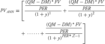
The present value of the annuity as of date 1 is denoted PVANN and defined to be:
The annual amount of the surplus or deficient payment is  . Dividing by PER to get the amount per period is a simplification because most FRNs use an actual/360 day count. Therefore, the amount typically would vary slightly from period to period but in this case it is constant.
Equation 7.1 contains the sum of a finite geometric series and can be reduced to equation 7.2:
PVANN is negative when QM < DM, meaning the quoted margin is deficient, most likely due to a credit downgrade or a loss in liquidity. Investors require a higher margin over the reference rate in order to pay par value on date 1, so the FRN trades at a discount. Similarly, PVANN is positive when QM > DM, so the floater trades at a premium.
The market value of the floater on date t—that is, the full price (including accrued interest)—is denoted MV. It is the forthcoming interest payment plus the price of the FRN on date 1, both discounted back over the remainder of the period at the yield per period.
Here you can see again that this is a simple model in that the same yield is used for all the discounted cash flows. You could argue that a better discount rate in equation 7.3 would be a short-term money market rate, but then the model is more complicated.
Combining equations 7.2 and 7.3 provides a general valuation formula for the floater, given the discount margin.
A formula for DM given the current market value is obtained by rearranging equation 7.4.
A payoff from building this simple model is to obtain a general formula for the Macaulay duration (MacDurFRN) of the floating-rate note for date t in the coupon period, as shown in equation 7.6. The details to the derivation are in the Technical Appendix, but in brief entail using calculus and algebra on the first derivative of MV in equation 7.4, given a change in the yield per period.
We'll get to a numerical example of this equation in the next section, but for now let's examine the expression. Substitute equation 7.3 into equation 7.6 and rearrange the middle term.
(7.7) 
While not obvious, the third term in parentheses is always positive—it's the Macaulay duration of a fixed-payment annuity maturing in  − 1 periods. Therefore, the sign of the Macaulay duration depends on the middle term. If QM = DM, PVANN = 0 and MacDurFRN = 1 − t/T. That is the standard result for a risk-free floater having no change in credit risk, liquidity, or taxation—the Macaulay duration is just the fraction of the period remaining until the next reset date. When QM < DM and PVANN < 0, it's possible for MacDurFRN to be negative, especially for long-term FRNs (so that
  is large) that are near a payment date (so that t/T nears 1). The corollary is that when QM > DM because of a credit upgrade, PVANN > 0 and MacDurFRN is greater than 1 − t/T.
Negative duration is a phenomenon of floaters that are trading at a deep enough discount below par value. But this is duration with respect to the benchmark yield. In deriving equation 7.6, I make the sly move of holding DM constant when taking the derivative of equation 7.4 with respect to a change in y. By implication, credit risk is unchanged. That is, the difference between QM and DM stays the same when the yield that is used to discount the amount of the deficiency or surplus is changed. Therefore, equation 7.6 delivers a statistic similar to curve duration in Chapter 6, the sensitivity of the bond's market value to a shift in the entire Treasury yield curve. In this simple model, the duration is the sensitivity to a single benchmark yield. We can see this better by looking at an actual floating-rate note.
An Actual Floater
On June 13, 2006, JP Morgan Chase Bank issued at par value a 10-year floating-rate note paying 3-month LIBOR + 0.33%. Figure 7.1 displays its Bloomberg FRN Pricing Analysis page (YAF) for settlement on August 31, 2010. Its market price is stated to be 92.61077—that's the flat price. At the last reset date on June 14, 2010, 3-month LIBOR was 0.53644%. Interest is paid quarterly (PER = 4), and at the beginning of the period there were 6 years to the maturity date, which is June 13, 2016 (Z = 6). This settlement date is 78 days into a 91-day period (t/T = 78/91).
Figure 7.1 Bloomberg FRN Pricing Analysis Page (YAF), JP Morgan Chase Floating-Rate Note
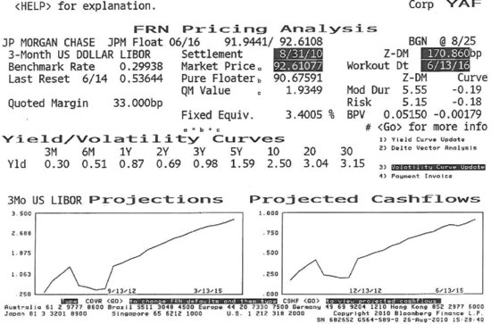
The interest payment due at the end of the quarter is 0.21902 per 100 of face value, calculated as  , where R0 = 0.0053644, QM = 0.0033, INT = 0.21902 and FV = 100. Typical of floaters, interest is calculated on an actual/360 basis. The accrued interest is the straight-line share of the forthcoming interest payment: 78/91* 0.21902 = 0.18773. The market value (MV) for the floater is 92.79850, the sum of the flat price and the accrued interest (92.79850 = 92.61077 + 0.18773).
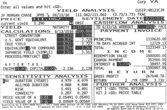
The remaining variable is the yield per period needed to discount the annuity representing the deficiency in the quoted margin. Obviously, a floating-rate note does not have a conventional yield statistic because the future cash flows are unknown. One solution is to project future levels of LIBOR and the corresponding interest payments and then solve for the internal rate of return. Luckily for us, JP Morgan Chase issued a companion 10-year, fixed-rate note at the same time it issued the floater. Its Bloomberg Yield Analysis (YA) page is shown in Figure 7.2. The street convention yield to maturity is 3.730% (s.a.). We need to convert that semiannual bond basis yield to quarterly compounding. Using the periodicity conversion equation 1.9 from Chapter 1, the corresponding yield is 3.7128%.

So, the yield per quarterly period, y, is 0.009282 (= 0.037128/4).
Figure 7.2 Bloomberg Yield Analysis Page (YA), JP Morgan Chase Fixed-Rate Note
This gives us the inputs for equation 7.6, noting that  .
.

That's the duration in terms of a change in the yield per quarter. Annualized, the Macaulay duration is −0.1919 (= −0.7677/4). The annual modified duration is −0.1902 (= −0.1919/1.009282). We have a case of negative duration.
Two modified duration statistics are reported for this floater on the right side of the Bloomberg YAF page in Figure 7.1: The Z-DM duration is 5.55 and the Curve duration is −0.19. Clearly, the closed-form formula replicates the Curve duration result. Bloomberg gets its statistics using the approximation formula for annual modified duration, as in Chapter 6. Before demonstrating that calculation, we first need to understand Z-DM—the zero-discount margin. The Bloomberg help page describes it in this manner:
The traditional analysis of floating rate notes revolves around the calculation of discount margin (DM). DM is an adjustment applied to the discount rate that equates the calculated price to the quoted price. On any reset date, if the DM equals the quoted margin, the FRN prices at par. If the issuer's credit has improved or deteriorated since the note was issued, the DM and QM diverge. To compute Z-DM, the implied zero curve is derived from the yield curve. Then the future values for the index are projected. These rates are used to imply the floating cash flows. Using these cash flows, the implied zero-rate for each payment date is obtained. The forward rates are used to discount the cash flows. Z-DM is the adjustment that must be applied to each forward rate so the modeled price matches the market.
In other words, it's pretty much a “black box” calculation for the user. Fortunately, the simple valuation model produces similar results.
The Z-DM for the JP Morgan Chase floater is reported to be 170.860 basis points. Using equation 7.5, the required discount margin is 174.5365 basis points.

The advantage of the simple model is that it is more transparent than the Bloomberg calculation because the inputs are readily observed, and it does not involve projected levels for LIBOR. However, it does not contain as much information about the shape of the yield curve. I've noticed in playing with the model that the DM produced by equation 7.5 gets closer to the Bloomberg Z-DM number when the underlying yield curve is flatter.
The Bloomberg help page also describes how the modified duration statistics are obtained: “Sensitivity measures are calculated by shifting the zero-discount margin (Z-DM) and the underlying yield curve (Curve) up and down by one basis point and measuring the resulting price changes.”
To illustrate this process, I first need to show that DM = 0.01745365 and the other inputs produce the initial market value, 92.79850, using equation 7.4.

This is no surprise at all because 7.4 and 7.5 are the same equation, just rearranged algebraically.
Now we raise DM by 1 basis point (0.0001) from 0.01745365 to 0.01755365.
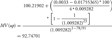
Then we lower DM by 1 basis point from 0.01745365 to 0.01735365.

These are the inputs to approximate the annual modified duration using equation 6.18 from Chapter 6, repeated here as equation 7.8.
Substitute the calculated values into equation 7.8 to get modified duration with respect to a change in the discount margin.

This rounds off to the Z-DM modified duration of 5.55 reported on the Bloomberg page.
Now we can carry out the same exercise, changing the yield but maintaining the same DM. First, raise the annual yield by 1 basis point (0.01%) from 3.7128% to 3.7228%, so the yield per quarter goes up from 0.009282 to 0.009307.

Then lower the annual yield by 1 basis point from 3.7128% to 3.7028%, so y drops from 0.009282 to 0.009257.

Plugging these values into equation 7.8 once again results in negative-duration with respect to the benchmark yield.

This approximation matches the closed-form equation and that reported on the Bloomberg page.
So, after all of this arduous bond math, what do we know about this JP Morgan Chase floater? First, it's trading at a discount because investors require a higher margin over 3-month LIBOR than 33 basis points. In fact, they require somewhere around 170 to 174 basis points, depending on the valuation model. Then, in theory, the floater would reprice at par value on each quarterly payment date. Second, this floater will respond very differently to a change in benchmark interest rates than to a change in credit or liquidity risk. Remember that on a traditional fixed-rate bond, the duration statistic signals the impact on market value from a given change in the yield to maturity, regardless of whether that change is due to a change in the benchmark yield or in the credit spread. That is, a fixed-rate bond's benchmark yield and credit spread duration statistics are equivalent. This is not so with a floating-rate bond.
The Bloomberg Z-DM duration of 5.55 indicates that a 100-basis point increase in the required margin over LIBOR should reduce the value of the floater by about 5.55%. However, I think that the Bloomberg statistic overstates this impact. Notice that in confirming that result I raised and lowered DM by 1 basis point but kept the yield the same. In my opinion, a better approach is also to raise and lower the annual yield by the same amount. Then we would be faithful to the idea of holding the benchmark yield constant while the credit spread changes. When I do that, I get an approximate annual modified duration of 5.36. In any case, the conclusion is that FRNs experience percentage changes in value similar to fixed-rate notes of comparable maturity when concerns over credit risk and liquidity are driving market prices.
The Bloomberg Curve modified duration of −0.19 indicates a small but surprising positively correlated response to a change in the benchmark yield curve. That's because the floater is trading at a discount. The amount of the discount is the present value of an annuity—the difference between the quoted margin and the required (or discount) margin. If credit quality deteriorates further, the annuity becomes larger and the price of the floater falls, just like a fixed-rate bond. If there is no further change in credit quality or liquidity, the size of the annuity remains the same. Then a higher benchmark yield reduces the present value of the annuity and the amount of the discount goes down. So, the floater's price goes up when the benchmark yield goes up—hence, negative duration. A lower benchmark yield raises the present value of the annuity, increasing the size of the discount. The price falls when the yield falls—again, negative duration.
Inflation-Indexed Bonds: C-Linkers and P-Linkers
The market for inflation-indexed bonds (linkers) has grown enormously in the last thirty years. P-Linkers, for which the coupon rate is fixed and the principal is linked to changes in the consumer price index (ΔCPI), are usually issued by governments. These include U.S. Treasury TIPS (Treasury Inflation-Protected Securities), which have been available since 1997 and borrowed their design from linkers issued in the United Kingdom (1981), Australia (1983), and Canada (1991). C-Linkers are essentially floating-rate notes for which the principal is fixed and the variable coupon rate is linked to the ΔCPI. They tend to be issued by commercial banks and life insurance companies.
While inflation-adjusted linkers might seem to be straightforward securities, they are quite complex in theory and in practice. That's because inflation is arbitrarily measured and reported. There are many conceptual and political issues: Whose “consumption bundle” is measured for month-to-month price changes? When and how should that bundle be re-weighted as new products are introduced and consumer spending patterns change? Should the bundle be adjusted when consumers substitute one good for another because of relative price changes? How should quality improvements be handled, that is, buying a better widget that costs more and not just the same old widget at an inflated price? How is the cost of residential housing (a major household budget item) measured and included in the CPI? Does it matter that government collects the data and calculates the official inflation rate that directly impacts the cost of its own debt? To focus on the bond math aspects of linkers, we'll neglect these issues and just assume that inflation is measured and reported accurately.
First, consider a highly stylized 2.50%, annual payment, 10-year P-Linker that adjusts the principal yearly based on the ΔCPI. In practice, TIPS make semiannual interest payments and adjust the principal for the 2-month lagged ΔCPI—that lag makes it difficult to model intra-period valuation. Table 7.1 shows the nominal and real cash flows for the P-Linker assuming a low-inflation scenario. The CPI starts at 100 on date 0 and rises for arbitrarily chosen values to 118.752 on date 10 for an average annual inflation rate of 1.734%, including a couple of years of deflation. Inflation is calculated as the percentage change in the CPI from one year to the next. For instance, the inflation rate of 2.863% for the tenth year is 118.752/115.447 − 1.
Table 7.1 2.50%, 10-Year, Annual Payment P-Linker, Low-Inflation Scenario
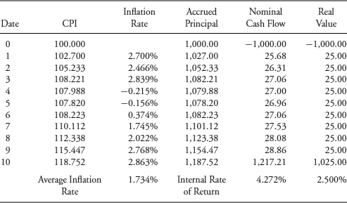
The accrued principal on a P-Linker is reported in Table 7.1 per $1,000 in par value. The key point is that the nominal interest payment each year is the fixed 2.50% coupon rate times the accrued principal. The $1,217.21 final payment at maturity is the accrued principal as of that date, $1,187.52, plus the interest payment, $29.69 (= 0.0250 * $1,187.52). The real value deflates the nominal cash flow for the cumulative increase in the CPI since the base year. For the final payment, $1,217.21 is divided by 118.752/100 to get a real value of $1,025.00. The internal rates of return (IRR) are calculated for the nominal and real values assuming purchase at par value for $1,000—the cash flow on date 0 is negative to indicate an outflow to the investor. I use the IRR financial function in Excel to get those results.
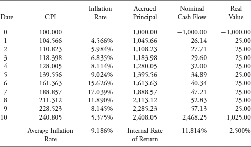
Table 7.2 repeats the exercise assuming a high-inflation scenario, where the CPI rises from 100 to 240.805, resulting in an average inflation rate of 9.186%. Obviously, the nominal IRR is much higher. The salient point is that the real values of the cash flows for each date and the real IRR, overall, are the same in each scenario. That is the essence of inflation protection—to provide a predictable rate of return in real (i.e., after inflation) terms (assuming no default, of course). Note that the real yield of 2.50% is not really “locked in” because there still is coupon reinvestment risk with respect to changes in future real rates of interest. Also, TIPS provide deflation protection as well because at maturity, the investor receives the accrued principal or par value, whichever is higher.
Table 7.2 2.50%, 10-Year, Annual Payment P-Linker, High-Inflation Scenario
Second, consider a stylized annual payment C-Linker paying 2.50% plus ΔCPI for the year. C-Linkers in practice often make monthly interest payments. Tables 7.3 and 7.4 show the nominal and real cash flows for the annual payment C-Linker purchased at par value for the same low- and high-inflation scenarios. On date 3 in Table 7.3, the inflation rate for the third year is determined to be 2.839%, making the coupon rate 5.339% (= 2.50% + 2.839%). The nominal interest payment is $53.39, the coupon rate times the constant principal amount of $1,000. The following year experiences deflation—in particular, an inflation rate of −0.215%. The coupon rate is 2.285% (= 2.50% − 0.215%). C-Linkers offer deflation protection in that the coupon rate will go no lower than zero if there is more than 2.50% deflation.
Table 7.3 2.50%, 10-Year, Annual Payment C-Linker Low-Inflation Scenario
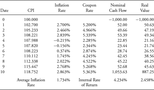
Table 7.4 2.50%, 10-Year, Annual Payment C-Linker High-Inflation Scenario
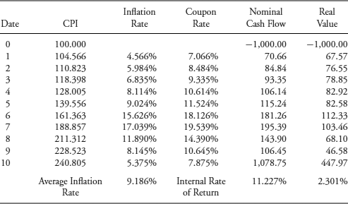
Notice that the cash flows are more “front-loaded” on the C-Linker than on the P-Linker. That is because the compensation for inflation on the C-Linker is paid as it is realized, whereas it is mostly deferred until maturity on the P-Linker. Three implications of this difference in the timing of cash flows are: (1) More coupon reinvestment risk with C-Linkers (more cash flow received sooner subject to fluctuation in real rates); (2) Higher real rate durations with P-Linkers (longer time to the receipt of cash flow); and (3) Less potential credit risk on C-Linkers, depending of course on the issuer (credit risk typically is an increasing function of time to the receipt of cash flow). These differences, along with taxation, are important when an investor has a choice between P-Linkers and C-Linkers.
Before turning to linker taxation, notice that the real IRR on the 2.50% C-Linker is lower than on the 2.50% P-Linker, even though both are purchased at par value. Given low inflation averaging 1.734%, the C-Linker underperforms by 4.2 basis points. For high inflation averaging 9.186%, the difference is 19.9 basis points. The reason for this is that the typical C-Linker does not provide complete inflation protection—the interest payment formula leaves out the cross-product between the inflation rate and the real rate in setting the nominal rate. Recall from Chapter 3 the relationship among the three rates: (1 + nominal rate) = (1 + real rate) * (1 + inflation rate). Multiplying the terms, this becomes: nominal rate = real rate + inflation rate + (real rate * inflation rate). The typical C-Linker only includes the first two terms.
Hopefully, investors are aware of the interest payment formula on typical C-Linkers and that deficiency is reflected in the market price, especially if high inflation rates are expected. In reality, some C-Linkers do include the cross-product. The U.S. Treasury issues retail-oriented Series I Savings Bonds (called I-Bonds). These non-marketable, 30-year C-Linkers can be purchased at par value in small denominations of $25. The coupon interest rate is reset semiannually based on the ΔCPI, including the cross-product. Interest accrues over the lifetime of the I-Bond and is paid at redemption. These, like P-Linkers, have the same real IRR for all subsequent paths for inflation. But that is before taxes.
Linker Taxation
This discussion of the taxation of inflation-indexed bonds is going to be simplistic, especially after the detail of Chapter 4. The stylized P-Linker and C-Linker are assumed to be purchased at par value and held to maturity. There are no capital gains or losses and no de minimis OID, just ordinary income tax. My objective is to demonstrate that these two designs offering inflation protection generate very different after-tax cash flows. Moreover, when the inflation rate is high, the after-tax real rates of return become negative. That explains why linkers usually are held in tax-deferred, retirement portfolios like defined-benefit and defined-contribution pension funds.
Table 7.5 shows the after-tax cash flows on the 2.50%, annual payment, 10-year P-Linker assuming a 30% tax rate on ordinary income and the high-inflation scenario. On date 6, the inflation rate for the year reaches double digits, 15.626%, raising the accrued principal up to $1,613.63 from $1,395.56. The interest payment is $40.34 (= 0.0250 * $1,613.63). The tax obligation on the interest income is $12.10 (= 0.30 * $40.34). But P-Linker taxation does not stop there—the increase in the accrued principal is taxed as ordinary income in the current year even though that compensation for inflation is not received until maturity. This is another example of phantom income. That tax is $65.42 [= 0.30 * ($1,613.63 − $1,395.56)]. The total tax obligation is $77.52 (= $12.10 + $65.42), resulting in an after-tax cash flow of −$37.18 (= $40.34 − $77.52).
Table 7.5 After-Tax Cash Flows on the 2.50%, 10-Year, Annual Payment P-Linker, High-Inflation Scenario, 30% Tax Rate
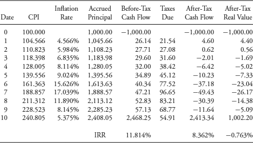
Negative after-tax cash flows for the P-Linker start in the third year and last until maturity in this high-inflation scenario. A useful calculation for the investor is the threshold inflation rate, shown in equation 7.9, which indicates the point at which negative after-tax cash flows arise. It's derived in the Technical Appendix.
Fixed Rate is the coupon rate on the P-Linker, here 2.50%, and Tax Rate is the applicable rate on ordinary income, here 30%. Substituting those into equation 7.9 gives a threshold rate of 6.195%.

In general, the lower the fixed coupon rate and the higher the tax rate, the lower is the threshold inflation rate that results in negative after-tax cash flow.
The after-tax cash flows for the 2.50%, annual payment, 10-year C-Linker are shown in Table 7.6 for the same high-inflation scenario. For the sixth year when the inflation rate is 15.626%, the coupon rate is set at 18.126% (= 2.50% + 15.626%) and the interest payment is $181.26 per $1,000 in par value. The tax obligation is $54.38 (= 0.30 * $181.26), leaving an after-tax cash flow of $126.88 (= $181.26 − $54.38). This is much more straightforward than the P-Linker—there is no taxable phantom income or negative after-tax cash flow.
Table 7.6 After-Tax Cash Flows on the 2.50%, 10-Year, Annual Payment C-Linker, High-Inflation Scenario, 30% Tax Rate
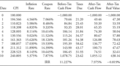
The sad news is that both of these linkers are projected to deliver negative after-tax real IRRs. To be sure, the realized real rates of return will depend on actual real rates when the coupons are reinvested. These results ultimately depend on the particular price and rate assumptions. It's easy to put these stylized linkers onto a spreadsheet to see the impact of lowering the purchase price, raising the fixed coupon rate, lowering the tax rate, and lowering the average inflation rate. Those changes raise the after-tax real IRR and can make it a positive outcome. For instance, other things being equal, if the tax rate is less than 23.04% on this 2.50%, 10-year P-Linker, and less than 22.21% on the C-Linker, the after-tax IRRs are above zero. An individual investor can manage the tax problem by holding the linker in a tax-deferred, retirement savings account like a 401(k) or 403(b). Doing so won't make the tax obligation go away, but will allow the investment to compound at the before-tax real yield.
Linker Duration
Yield duration in Chapter 6 is defined as the sensitivity of the fixed-income bond price to a change in the nominal yield to maturity. Inflation-indexed bonds require that we focus on why the nominal rate changes and distinguish between a change in the real rate and a change in the inflation rate. Let's start by formalizing the stylized linkers, keeping close to the notation of Chapter 3. Let the nominal rate be y, the real rate r, and the inflation rate i. Also, let the number of periods to maturity be N, the fixed coupon rate c, the par (or face) value of the linker FV, and the current price PV. For these stylized linkers, we are on a coupon payment date so there is no accrued interest to sully the equations.
P-Linker valuation is based on the assumed path for the accrued principal. Given a constant inflation rate, this path will be  ,
,  . Then the price of the P-Linker, denoted PVPLINK, is the present value of the cash flows, discounted at the nominal rate.
(7.10) 
This equation is simplified using the standard relationship among the nominal, real, and inflation rates:  .
.
This can be written more compactly as shown in equation 7.12.
The inflation rate drops out in equations 7.11 and 7.12, so the inflation duration for the stylized P-Linker is zero. That's because the first derivative of the pricing equation with respect to a change in the inflation rate is zero. In practice, the time between measuring the ΔCPI and changing the accrued principal (i.e., the indexation lag) matters, and the inflation duration for TIPS is close to but not exactly zero.
In equation 7.12, only changes in the real rate impact the market value of the P-Linker. Its Macaulay duration, derived in the Technical Appendix and denoted RealMacDurPLINK in equation 7.13, is going to look familiar to you.
This is the same as equation 6.15 for the Macaulay duration of a standard fixed-rate bond on a coupon date (when  ). Real rate durations on TIPS are relatively high compared to Treasury notes and bonds for the same maturity because their fixed coupon rates and the real yields are relatively low. In general, the Macaulay yield duration statistic is inversely related to both the coupon rate and yield to maturity.
The present value of the C-Linker, PVCLINK, assuming a constant inflation rate, is shown in equation 7.14.
The principal is fixed and the inflation rate simply is added to the fixed coupon rate without the cross-product term. The projected cash flows again are discounted using the nominal rate. In closed-form, this reduces to equation 7.15.
The real rate Macaulay duration for the C-Linker (RealMacDurCLINK) is derived in the Technical Appendix. It entails taking the first derivative of equation 7.15 with respect to changes in r, which is contained in y, and doing some algebraic manipulation.
This equation has a similar structure to equation 7.13 for the P-Linker (and to equation 6.15 for the traditional fixed-rate bond). The key point is that, unlike the P-Linker, the real rate duration of the C-Linker is a function of the inflation rate, which enters the equation directly as i and indirectly in y. This will matter in Chapter 10 when we get to strategies, in particular, an immunization strategy that rests on matching the duration of the bond portfolio to some target. It will be much easier to implement such a strategy using P-Linkers than with C-Linkers.
The inflation Macaulay duration for the C-Linker (InflationMacDurCLINK) will turn out to be low but not equal to zero, even for these stylized securities. Equation 7.17 is derived in the Technical Appendix.
Notice that the first two terms are the same as RealMacDurCLINK. The third term reduces InflationMacDurCLINK—sometimes all the way into negative territory. Some numerical examples will establish the circumstances when negative inflation duration occurs. It's not obvious from looking at equation 7.17.
Suppose that someday an inspired government offers a full array of long-term P-Linkers and C-Linkers. Perhaps this is to allow individuals to build low-risk retirement portfolios protected from inflation and deflation and hold them as either tax-deferred or currently taxable investments. Or perhaps the government seeks to assure holders of its traditional fixed-income debt that it has no intention of “inflating” its way out of its obligations. Assume that at present there are 20-year, annual payment P-Linkers and C-Linkers having coupon rates of 1.00%, 2.50%, and 4.00%. Investors require a real rate of 2.50%, so the 1.00% linkers trade at substantial discounts and the 4.00% linkers at substantial premiums. Assume that they originally were issued as 25-year or 30-year securities at par value and since then the real rates have been volatile. The 2.50%, 20-year linkers are the newly issued on-the-run offerings.
Table 7.7 shows the prices and Macaulay durations for these 20-year linkers given two inflation rates, 1.00% and 4.00%. For the real rate of 2.50%, the nominal rates are 3.525% (= 1.0250 * 1.01 − 1) and 6.60% (= 1.0250 * 1.04 − 1). The prices and durations are calculated by substituting N = 20, FV = 100, r = 0.0250, i = 0.01 or 0.04, y = 0.03525 or 0.0660, and c = 0.01, 0.0250, or 0.04 into equations 7.12, 7.13, 7.15, 7.16, and 7.17 (using a spreadsheet). There is a lot going on these numerical examples, so it is worthwhile examining them closely.
Table 7.7 Prices and Real Rate and Inflation Macaulay Duration Statistics on 20-Year P-Linkers and C-Linkers
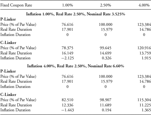
First, notice that the prices and durations for the P-Linker are the same for both inflation rates. The Macaulay real rate durations are high, given the 20-year time to maturity, and are inversely related to the fixed coupon rate (as is a traditional fixed-rate bond). The modified real rate durations are easily calculated. For instance, the modified duration for the 1%, 20-year P-Linker is 17.464 (= 17.901/1.025). The inflation durations are all zero.
You might be questioning these prices for the P-Linker, thinking that if expected future inflation were to jump suddenly from 1.00% to 4.00%, the prices of P-Linkers such as TIPS surely would react. The demand for inflation-protected securities would go up, driving their prices up and the real rate down. So, if a change in inflation impacts the price of the P-Linker, how could its inflation duration be zero? Good point. Table 7.7 implicitly assumes that the real rate remains the same whereas your analysis has the real rate changing. However, how much so is estimated by the real rate duration statistic, not the inflation duration. Suppose you figure that the heightened demand for linkers will reduce the real rate by 10 basis points from 2.50% to 2.40%. The price of the 4%, 20-year P-Linker would go up from 123.384 by approximately 1.780, estimated by the modified real rate duration times the price times the change in the real rate.

The key point is that these real rate and inflation duration statistics are what we call comparative static properties of the security—we assume other variables are held constant when we change one in particular. In reality, when the nominal interest rate goes up or down, both inflation and real rates change as well, but not necessarily by the same amount or in the same direction or in any consistent manner. One way of dealing with this is to calculate the duration of the linker with respect to the nominal rate and just assume some breakdown between the two component rates. That breakdown sometimes is called the “yield beta.” For example, if you assume a yield beta of 0.50, you would get a nominal Macaulay duration for the 4% P-Linker of 7.393 (= 14.786/2). That means you assume that a 1.00% change in the nominal rate is half due to inflation and that the other half is attributable to the real rate. In my opinion, this is a rather ad hoc approach. I think it is more insightful to work with the underlying real rate and inflation duration statistics.
Notice that the prices on the 2.50% C-Linker are less than par value even though the real rate is also 2.50%. That's because of the absence of the cross-product term. This effect is heightened when the inflation rate is higher. The real rate durations for the C-Linkers are high but still are lower than the corresponding P-Linker because, by design, the compensation for inflation is more “front-loaded.” That reduces the weighted-average time to the receipt of cash flow. Importantly, we now see that negative inflation duration occurs when the C-Linker is trading at a price sufficiently below par value.
The reason why discount C-Linkers have negative inflation duration and why premium C-Linkers have positive inflation duration is that they fundamentally are floating-rate notes. Their real rate durations are like the Z-DM duration on a traditional floater; their inflation durations are like Curve duration. The key difference is the location of the real rate. With a floater, it's in the nominal money market reference rate. With a C-Linker, it's in the fixed coupon rate along with compensation for credit and liquidity risk.
When the real rate goes up, the C-Linker trades at a discount. The amount of the discount is the present value of the annuity representing the deficiency in the fixed coupon. If there is no further change in the real rate, a drop in the inflation rate lowers the nominal rate used to get that present value. A lower discount rate increases the present value of the annuity, increasing the amount of the discount and lowering the price of the C-Linker. In sum, a lower inflation rate reduces the price—that's negative inflation duration.
Not understanding the inflation duration of C-Linkers could lead to real surprises for aggressive traders positioning a portfolio based on an expected level of inflation. Suppose that the trader's view is that inflation will go up by more than is generally expected by other market participants. Normally the trader is not particularly concerned whether bonds are trading at a discount or a premium. With C-Linkers, however, it definitely does matter—the trader would want to hold low-coupon C-Linkers trading at a discount and having negative inflation duration. If the view is toward lower-than-expected inflation, the trader prefers high-coupon, premium C-Linkers having positive inflation duration. Of course, the trader in each case also has to factor in the likely impact on real rates and use the real rate duration to assess the additional price change.
Conclusion
Floating-rate notes and inflation-indexed bonds demonstrate how we can employ a toolkit of bond math techniques to go beyond basic fixed-rate and zero-coupon securities. We have to extend our duration analysis to assess why the required rate of return changes and how that impacts market value. For floaters, changes in credit spreads and benchmark yields impact market value differently. For linkers, changes in the real rate and inflation have different impacts. Best of all, we can understand why and when floaters and linkers have negative duration. Now we can use the toolkit to delve into derivatives and the most commonly used product to manage fixed-income portfolios of assets or liabilities—interest rate swaps.
