Chapter 8
Learning Data Analysis Techniques
Highlight Cells That Meet Some Criteria
A conditional format is formatting that Excel applies only to cells that meet the criteria you specify. For example, you can tell Excel to apply only the formatting if a cell’s value is greater than or less than some specified amount, between two specified values, or equal to some value. You can also look for cells that contain specified text, dates that occur during a specified timeframe, and more.
When you set up your conditional format, you can specify the font, border, and background pattern. This helps to ensure that the cells that meet your criteria stand out from the other cells in the range.
Highlight Cells That Meet Some Criteria
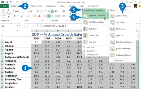
 Select the range you want to work with.
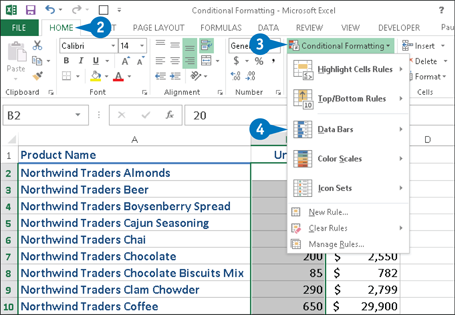
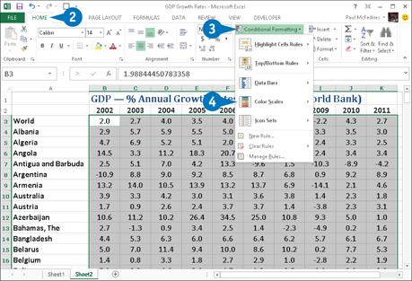
 Click the Home tab.
 Click Conditional Formatting.
 Click Highlight Cells Rules.
 Click the operator you want to use for the condition.
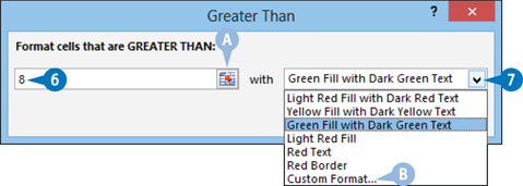
A dialog box appears with a name corresponding to the operator you clicked in step 5.
 Type the value to use for the condition.
A You can also click here and then click a worksheet cell.
Depending on the operator, you may need to specify two values.
 Click the down arrow and then click the formatting to use.
B To create your own format, click Custom Format.
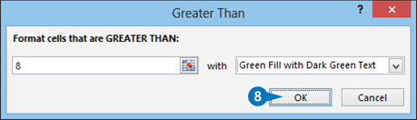
 Click OK.
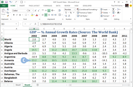
C Excel applies the formatting to cells that meet the condition you specified.
Highlight the Top or Bottom Values in a Range
When analyzing worksheet data, it is often useful to look for items that stand out from the norm. For example, you might want to know which sales reps sold the most last year, or which departments had the lowest gross margins. To view the extreme values in a range quickly and easily, you can apply a conditional format to the top or bottom values of that range.
You can do this by setting up top/bottom rules, where Excel applies a conditional format to those items that are at the top or bottom of a range of values. For the top or bottom values, you can specify a number, such as the top 5 or 10, or a percentage, such as the bottom 20 percent.
Highlight the Top or Bottom Values in a Range
Select the range you want to work with.
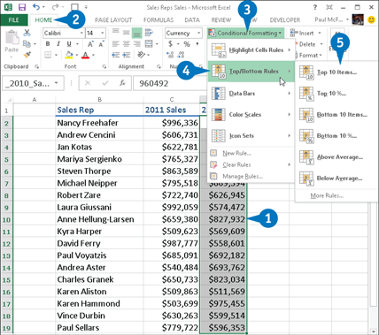
Click the Home tab.
Click Conditional Formatting.
Click Top/Bottom Rules.
Click the type of rule you want to create.
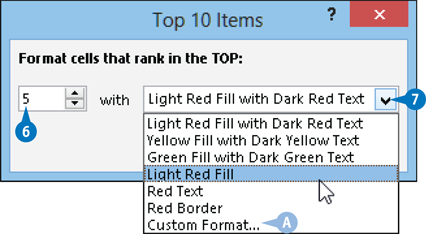
A dialog box appears with a name corresponding to the type of rule you clicked in step 5.
Type the value you want to use for the condition.
Click the down arrow and then click the formatting you want to use.
A To create your own format, click Custom Format.
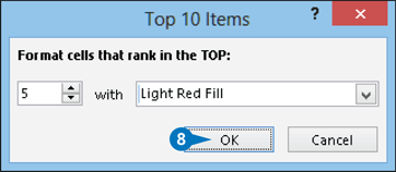
Click OK.
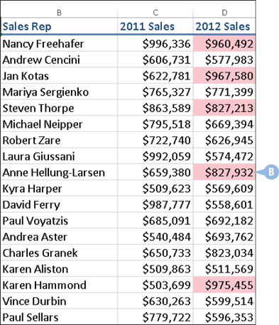
B Excel applies the formatting to cells that meet the condition you specified.
Show Duplicate Values
Excel can apply a conditional format to cells that meet the criteria you specify. You mostly use conditional formatting to highlight numbers greater than or less than some value, or dates occurring within some range. However, you can also use conditional formatting to look for duplicate values in a range.
Many range or table columns require unique values. For example, a column of student IDs or part numbers should not have duplicate values. With conditional formatting, you can specify a font, border, and background pattern that helps to ensure that any duplicate cells in a range or table stand out from the other cells.
Show Duplicate Values

Select the range you want to work with.
Click the Home tab.
Click Conditional Formatting.
Click Highlight Cells Rules.
Click Duplicate Values.
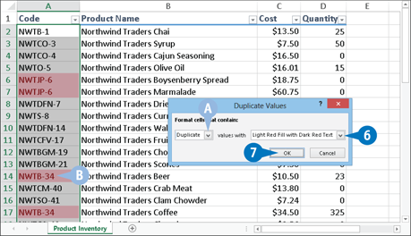
A dialog box appears with a name corresponding to the operator you clicked in step 5.
A To highlight the unique values in the range, click the down arrow, and then click Unique.
Click the down arrow and then click the formatting to use.
To create your own format, click Custom Format.
Click OK.
B Excel applies the formatting to any cells that have duplicate values in the range.
Show Cells That Are Above or Below Average
When you create top/bottom rules that apply a conditional format to cells at the top or bottom of a range of values, you mostly use these rules on either raw values or percentages. However, Excel also enables you to create top/bottom rules based on the average value in the range.
Specifically, you can highlight values that are either above or below the average of all the values in the range. You can specify a font, border, and background pattern that helps to ensure that these values stand out from the other cells.
Show Cells That Are Above or Below Average
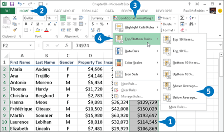
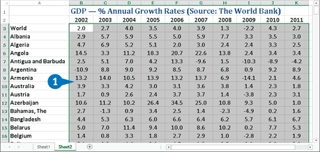
Select the range you want to work with.
Click the Home tab.
Click Conditional Formatting.
Click Top/Bottom Rules.
Click either Above Average or Below Average.
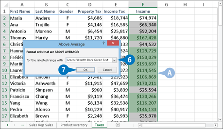
A dialog box appears with a name corresponding to the type of rule you clicked in step 5.
Click the down arrow and then click the formatting you want to use.
To create your own format, click Custom Format.
Click OK.
A Excel applies the formatting to cells that are either above or below average.
Analyze Cell Values with Data Bars
In some data analysis scenarios, you might be interested more in the relative values within a range than the absolute values. For example, if you have a table of products that includes a column showing unit sales, you may want to compare the relative sales of all the products.
This sort of analysis is often easiest if you visualize the relative values. You can do that by using data bars, a data visualization feature that applies colored, and horizontal bars to each cell in a range of values — these bars appear behind the values in the range. The length of the data bar that appears in each cell depends on the value in that cell: the larger the value, the longer the data bar.
Analyze Cell Values with Data Bars
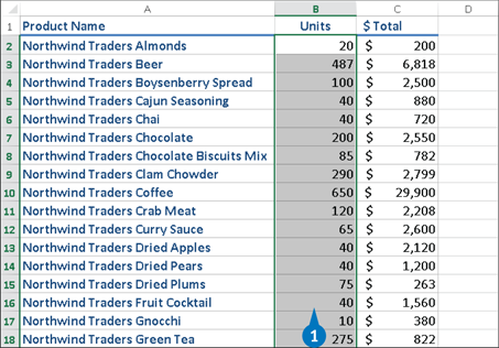
Select the range you want to work with.
Click the Home tab.
Click Conditional Formatting.
Click Data Bars.
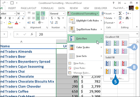
Click the fill type of data bars you want to create.
A Gradient fill data bars begin with a solid color and then gradually fade to a lighter color.
B Solid fill data bars are a solid color.
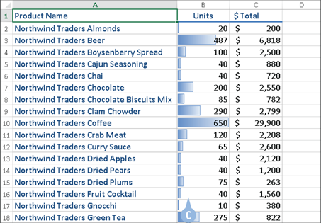
C Excel applies the data bars to each cell in the range.
Analyze Cell Values with Color Scales
It is often useful to get some idea about the overall distribution of values in a range. For example, you might want to know whether a range has many low values and just a few high values. Color scales can help you analyze your data in this way. A color scale compares the relative values in a range by applying shading to each cell, where the color reflects each cell’s value.
Color scales can also tell you whether your data includes outliers, values that are much higher or lower than the others are. Similarly, color scales can help you make value judgments about your data. For example, high sales and low numbers of product defects are good, whereas low margins and high employee turnover rates are bad.
Analyze Cell Values with Color Scales
Select the range you want to work with.
Click the Home tab.
Click Conditional Formatting.
Click Color Scales.
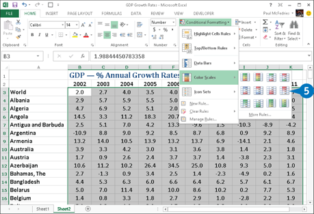
Click the color scale that has the color scheme you want to apply.
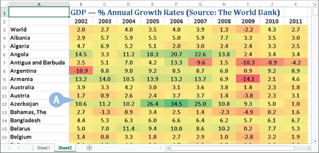
A Excel applies the color scales to each cell in the range.
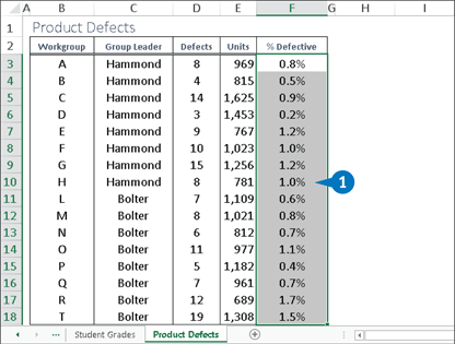
Analyze Cell Values with Icon Sets
You can help analyze large sets of data by applying to each cell an icon that has a symbolic association. This gives you a visual clue about the cell’s relative value compared with the overall distribution of values in the range.
Symbols that have common or well-known associations are often useful for analyzing large amounts of data. For example, a check mark usually means something is good, finished, or acceptable, whereas an X means something is bad, unfinished, or unacceptable. Similarly, a green circle is positive, whereas a red circle is negative (think traffic lights). Excel puts these and other symbolic associations to good use with the icon sets feature. You use icon sets to visualize the relative values of cells in a range.
Analyze Cell Values with Icon Sets

Select the range you want to work with.

Click the Home tab.
Click Conditional Formatting.
Click Icon Sets.

Click the type of icon set you want to apply.
The categories include Directional, Shapes, Indicators, and Ratings.
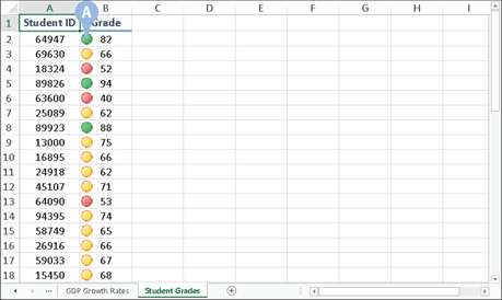
A Excel applies the icons to each cell in the range.
Create a Custom Conditional Formatting Rule
The conditional formatting rules in Excel — highlight cells rules, top/bottom rules, data bars, color scales, and icon sets — offer an easy way to analyze data through visualization. You can tailor your format-based data analysis by creating a custom conditional formatting rule that suits how you want to analyze and present the data.
These predefined rules do not suit particular types of data or data analysis. For example, the icon sets assume that higher values are more positive than lower values, but that is not always true. To get the type of data analysis you prefer, you can create a custom conditional formatting rule and Apply It to your range.
Create a Custom Conditional Formatting Rule
Select the range you want to work with.
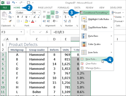
Click the Home tab.
Click Conditional Formatting.
Click New Rule.
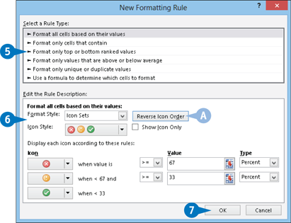
The New Formatting Rule dialog box appears.
Click the type of rule you want to create.
Edit the rule’s style and formatting.
The controls you see depend on the rule type you selected.
A With Icon Sets, click Reverse Icon Order if you want to reverse the normal icon assignments, as shown here.
Click OK.
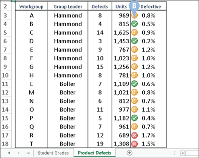
B Excel applies the conditional formatting to each cell in the range.
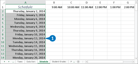
Highlight Cells Based On a Formula
You can also apply conditional formatting based on the results of a formula. In particular, you set up a logical formula as the conditional formatting criteria. For each cell where that formula returns TRUE, Excel applies the formatting you specify; for all the other cells, Excel does not apply the formatting.
In most cases, you use a comparison formula, or you use an IF function, often combined with another logical function such as AND or OR. In each case, your formula’s comparison value must reference only the first value in the range. For example, if the range you are working with is a set of dates in A2:A100, the comparison formula =WEEKDAY(A2)=6 would apply conditional formatting to every cell in the range that occurs on a Friday.
Create a Custom Conditional Formatting Rule
Select the range you want to work with.
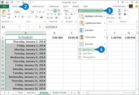
Click the Home tab.
Click Conditional Formatting.
Click New Rule.
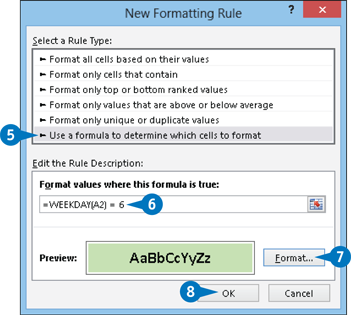
The New Formatting Rule dialog box appears.
Click Use a Formula to Determine Which Cells to Format.
Type the logical formula.
Edit the rule’s style and formatting.
Click OK.
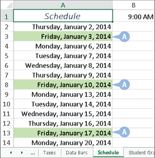
A Excel applies the conditional formatting to each cell in the range where the logical formula returns TRUE.
Modify a Conditional Formatting Rule
Conditional formatting rules are excellent data visualization tools that can make it easier and faster to analyze your data. Whether it is highlighting cells based on criteria, showing cells that are in the top or bottom of the range, or using features such as data bars, color scales, and icon sets, conditional formatting enables you to interpret your data quickly. Based on this, you might find that the conditional formatting you used was not correct because it does not enable you to visualize your data the way you had hoped. Similarly, a change in data might require a change in criteria. Whatever the reason, you can modify your conditional formatting rules to ensure you get the best visualization for your data.
Modify a Conditional Formatting Rule

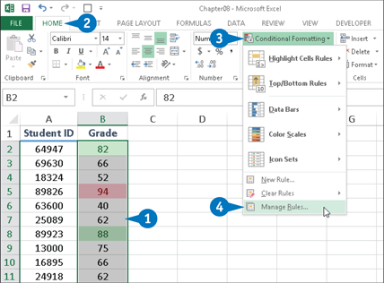
Select the range that includes the conditional formatting rule you want to modify.
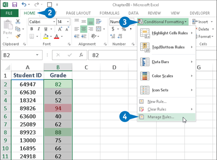
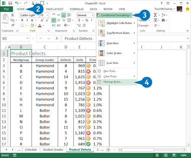
Click the Home tab.
Click Conditional Formatting.
Click Manage Rules.
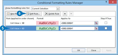
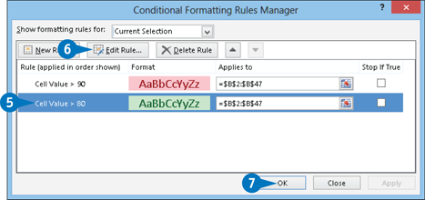
The Conditional Formatting Rules Manager dialog box appears.
Click the rule you want to modify.
Click Edit Rule.
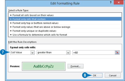
The Edit Formatting Rule dialog box appears.
Make your changes to the rule.
Click OK.
Excel returns you to the Conditional Formatting Rules Manager dialog box.
 Click OK (not shown).
Excel updates the conditional formatting.
EXTRA
If you have multiple conditional formatting rules applied to a range, the visualization is affected by the order in which Excel applies the rules. Specifically, if a cell already has a conditional format applied, Excel does not overwrite that format with a new one. For example, suppose you have two conditional formatting rules applied to a list of student grades: one for grades over 90 and one for grades over 80. If you apply the over-80 conditional format first, Excel will never apply the over-90 format because those values are already covered by the over-80 format. To fix this, in the Conditional Formatting Rules Manager dialog box, click the rule you want to modify, and then click the Move down ( ) or Move Up (
 ) sort button to set the order.
Remove Conditional Formatting from a Range
Conditional formatting rules are useful data visualization tools that make it easier to perform certain types of data analysis. For example, if your data is essentially random, then conditional formatting rules will not enable you to see patterns in that data. You might also find that conditional formatting is not helpful for certain collections of data or certain types of data. On the other hand, you might find conditional formatting useful for getting a handle on your data set, but then prefer to remove the formatting. If, for whatever reason, you find that a range’s conditional formatting is not helpful or no longer required, you can remove the conditional formatting from that range.
Remove Conditional Formatting from a Range
Select the range you want to work with.
Click the Home tab.
Click Conditional Formatting.
Click Manage Rules.
If you have multiple rules defined and you want to remove them all, click Clear Rules and then click Clear Rules from Selected Cells.
The Conditional Formatting Rules Manager dialog box appears.
Click the rule you want to remove.
Click Delete Rule.
Excel removes the rule from the range.
Click OK.
Remove Conditional Formatting from a Worksheet
Although the data visualization aspect of conditional formatting rules is part of the appeal of this Excel feature, as with all things visual it is possible to overdo it. That is, you might end up with a worksheet that has multiple conditional formatting rules and therefore some unattractive and confusing combinations of highlighted cells, data bars, color scales, and icon sets.
If you find that a worksheet’s conditional formatting is hindering your data analysis efforts rather than helping them, you can remove conditional formatting from that worksheet. You can either remove individual conditional formatting rules or clear the worksheet of all its conditional formatting.
Remove Conditional Formatting from a Worksheet
Select the worksheet.
Click the Home tab.
Click Conditional Formatting.
Click Manage Rules.
If you have multiple rules defined and you want to remove them all, click Clear Rules and then click Clear Rules from Entire Sheet.
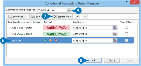
The Conditional Formatting Rules Manager dialog box appears.
Click the Show Formatting Rules For down arrow and select This Worksheet.
Click the rule you want to remove.
Click Delete Rule.
Excel removes the rule from the worksheet.
Click OK.
Set Data Validation Rules
You can make Excel data entry more efficient by setting up data entry cells to accept only certain values. To do this, you can set up a cell with data validation criteria that specify the allowed value or values. This is called a data validation rule. You can work with numbers, dates, times, or even text length, and you can set up criteria that are between two values, equal to a specific value, greater than a value, and so on.
Excel also lets you tell the user what to enter by defining an input message that appears when the user selects the cell. You can also configure the data validation rule to display a message when the user tries to enter an invalid value.
Set Data Validation Rules
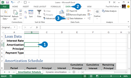
Click the cell you want to restrict.
Click the Data tab.
Click Data Validation.
The Data Validation dialog box appears.
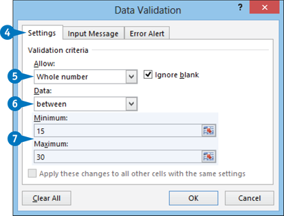
Click the Settings tab.
Click the Allow down arrow and select the type of data to allow in the cell.
Click the Data down arrow and select the operator to use to define the allowable data.
Specify the validation criteria, such as the Minimum and Maximum allowable values shown here.
Note: The criteria boxes you see depend on the operator you chose in step 6.
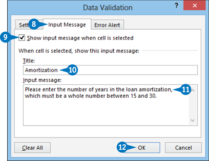
Click the Input Message tab.
Click the Show Input Message When Cell Is Selected check box if it is not selected ( changes to
  ).
).
 Type a message title in the Title text box.
 Type the message you want to display in the Input Message text box.
 Click OK.
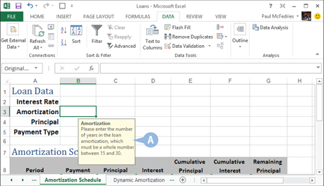
Excel configures the cell to accept only values that meet your criteria.
A When the user selects the cell, the input message appears.
APPLY IT
You can configure the cell to display a message if the user tries to enter an invalid value. Follow steps 1 to 3 to open the Data Validation dialog box, and then click the Error Alert tab. Make sure the Show Error Alert After Invalid Data Is Entered check box is selected (), and then specify the Style, Title, and Error Message. Click OK.
If you no longer need to use data validation on a cell, you should clear the settings. Follow steps 1 to 3 to display the Data Validation dialog box and then click Clear All. Excel removes all the validation criteria, as well as the input message and the error alert. Click OK.
Summarize Data with Subtotals
Although you can use formulas and worksheet functions to summarize your data in various ways — including sums, averages, counts, maximums, and minimums — if you are in a hurry, or if you just need a quick summary of your data, you can get Excel to do the work for you. The secret here is a feature called automatic subtotals, formulas that Excel adds to a worksheet automatically.
Excel sets up automatic subtotals based on data groupings in a selected field. For example, if you ask for subtotals based on the Customer field, Excel runs down the Customer column and creates a new subtotal each time the name changes. To get useful summaries, you can sort the range on the field containing the data groupings in which you are interested.
Summarize Data with Subtotals
Click a cell within the range you want to subtotal.
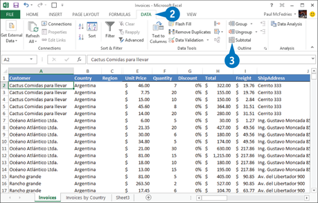
Click the Data tab.
Click Subtotal.
The Subtotal dialog box appears.
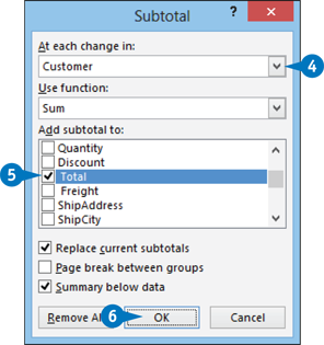
Click the down arrow and then click the column you want to use to group the subtotals.
In the Add Subtotal To list, click the check box for the column you want to summarize ( changes to ).
Click OK.
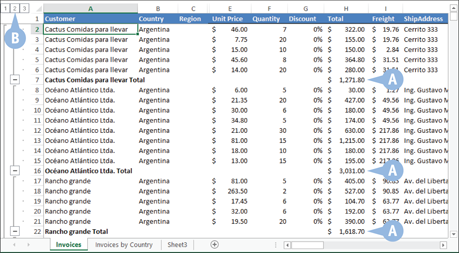
A Excel calculates the subtotals and adds them into the range.
B Excel adds outline symbols to the range.
Note: See the next section, Group Related Data, to learn more about outlining in Excel.
Group Related Data
To help you analyze a worksheet, you can control a worksheet range display by grouping the data based on the worksheet formulas and data. Grouping the data creates a worksheet outline, which works similarly to the outline feature in Microsoft Word. In a worksheet outline, you can collapse sections of the sheet to display only summary cells (such as quarterly or regional totals), or expand hidden sections to show the underlying detail. Note that when you add subtotals to a range, Excel automatically groups the data and displays the outline tools. For more information, see the section, Summarize Data with Subtotals.
Group Related Data
Create the Outline

Display the worksheet you want to outline.
Click the Data tab.
Click the Group down arrow.
Click Auto Outline.
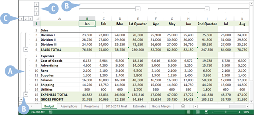
A Excel outlines the worksheet data.
B Excel uses level bars to indicate the grouped ranges.
C Excel displays level symbols to indicate the various levels of the detail that are available in the outline.
Use the Outline to Control the Range Display
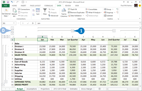
Click a Collapse symbol to hide the range indicated by the level bar.
D You can also collapse multiple ranges that are on the same outline level by clicking the appropriate level symbol.

E Excel collapses the range.
Click the Expand symbol to view the range again.
F You can also show multiple ranges that are on the same outline level by clicking the appropriate level symbol.
Remove Duplicate Values from a Range or Table
You can make your Excel data more accurate for analysis by removing any duplicate records. Duplicate records throw off your calculations by including the same data two or more times. To prevent this, you should delete duplicate records. Rather than looking for duplicates manually, you can use the Remove Duplicates command, which can quickly find and remove duplicates in even the largest ranges or tables.
Before you use the Remove Duplicates command, you must decide what defines a duplicate record in your data. That is, you must specify whether every field has to be identical or whether it is enough that only certain fields are identical.
Remove Duplicate Values from a Range or Table
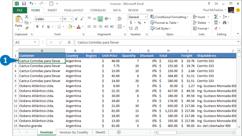
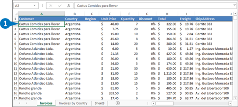
Click a cell inside the range or table.

Click the Data tab.
Click Remove Duplicates.
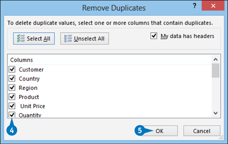
The Remove Duplicates dialog box appears.
Click the check box beside each field that you want Excel to check for duplication values( changes to ).
Note: Excel does not give you a chance to confirm the deletion of the duplicate records, so be sure you want to do this before proceeding.
Click OK.
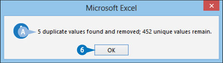
Excel deletes any duplicate records that it finds.
A Excel tells you the number of duplicate records that it deleted.
Click OK.
APPLY IT
If your data has many columns, you may want Excel to use only one or two of those fields to look for duplicates. To make this easier, first click Unselect All in the Remove Duplicates dialog box to clear all the check boxes; then select just the check boxes you want Excel to use.
To remove duplicates when your range does not have column headers, open the Remove Duplicates dialog box and deselect the My Data Has Headers check box ( changes to ). Use the check boxes labeled Column A, Column B, and so on to choose the columns that you want Excel to check for duplicate values.
Consolidate Data from Multiple Worksheets
Companies often distribute similar worksheets to multiple departments to capture budget numbers, inventory values, survey data, and so on. Those worksheets must then be combined into a summary report showing company-wide totals. This is called consolidating the data.
Rather than doing this manually, Excel can consolidate your data automatically. You can use the Consolidate feature to consolidate the data either by position or by category. In both cases, you specify one or more source ranges (the ranges that contain the data you want to consolidate) and a destination range (the range where the consolidated data will appear).
Consolidate Data from Multiple Worksheets
Consolidate by Position
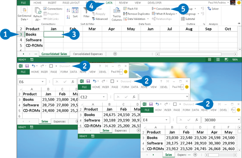
Create a new worksheet that uses the same layout — including row and column headers — as the sheets you want to consolidate.
Open the workbooks that contain the worksheets you want to consolidate.
Select the upper-left corner of the destination range.
Click the Data tab.
Click Consolidate.
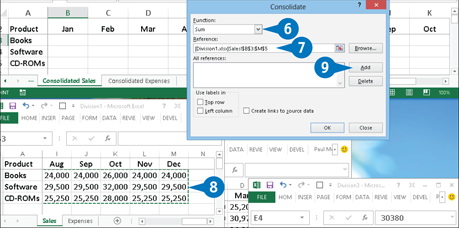
The Consolidate dialog box appears.
Click the Function down arrow and then click the summary function you want to use.
Click inside the Reference text box.
Select one of the ranges you want to consolidate.
Click Add.
A Excel adds the range to the All References list.
Repeat steps 7 to 9 to add all of the consolidation ranges.
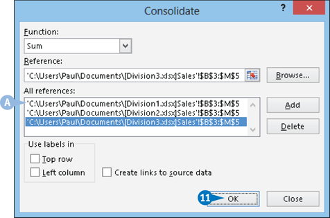
Click OK.
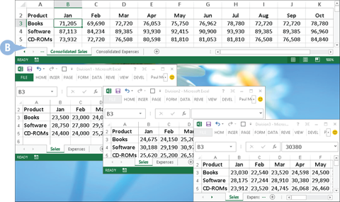
B Excel consolidates the data from the source ranges and displays the summary in the destination range.
APPLY IT
If the source data changes, then you probably want to reflect those changes in the consolidation worksheet. Rather than running the entire consolidation over again, a much easier solution is to click the Create Links to Source Data check box ( changes to ) in the Consolidate dialog box. This enables you to update the consolidation worksheet by clicking the Data tab and then clicking Refresh All.
This also means that Excel creates an outline in the consolidation sheet, and you can use that outline to see the detail from each of the source ranges. See the section, Group Related Data to learn more about outlines in Excel.
If the worksheets you want to summarize do not use the same layout, you need to tell Excel to consolidate the data by category. This method consolidates the data by looking for common row and column labels in each worksheet. For example, suppose you are consolidating sales. Division A sells software, books, and videos. Division B sells books and CD-ROMs. Division C sells books, software, videos, and CD-ROMs. When you consolidate this data, Excel summarizes the software and videos from Divisions A and C, the CD-ROMs from Divisions B and C, and the books from all three.
Consolidate Data from Multiple Worksheets
Consolidate by Category
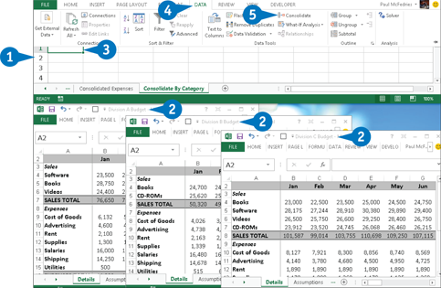
Create a new worksheet for the consolidation.
Open the workbooks that contain the worksheets you want to consolidate.
Select the upper-left corner of the destination range.
Click the Data tab.
Click Consolidate.
The Consolidate dialog box appears.
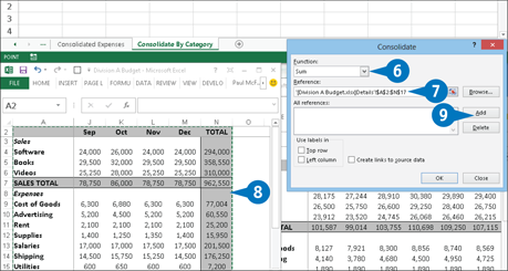
Click the Function down arrow and then click the summary function you want to use.
Click inside the Reference text box.
Select one of the ranges you want to consolidate.
Note: Be sure to include the row and column labels in the range.
Click Add.
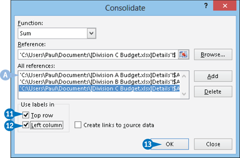
A Excel adds the range to the All References list.
Repeat steps 7 to 9 to add all of the consolidation ranges.
If you have labels in the top row of each range, click the Top Row check box to select it ( changes to ).
If you have labels in the left-column row of each range, click the Left Column check box to select it ( changes to ).
 Click OK.
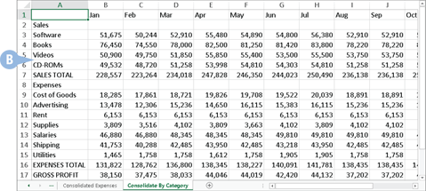
B Excel consolidates the data from the source ranges and displays the summary in the destination range.