We discuss the simple yet powerful ideas which have allowed to break the diffraction resolution limit of lens-based optical microscopy. The basic principles and standard implementations of STED (stimulated emission depletion) and RESOLFT (reversible saturable/switchable optical linear (fluorescence) transitions) microscopy are introduced, followed by selected highlights of recent advances, including MINFLUX (minimal photon fluxes) nanoscopy with molecule-size (~1 nm) resolution.
We are all familiar with the sayings “a picture is worth a thousand words” and “seeing is believing”. Not only do they apply to our daily lives, but certainly also to the natural sciences. Therefore, it is probably not by chance that the historical beginning of modern natural sciences very much coincides with the invention of light microscopy . With the light microscope mankind was able to see for the first time that every living being consists of cells as basic units of structure and function; bacteria were discovered with the light microscope, and also mitochondria as examples of subcellular organelles.
However, we learned in high school that the resolution of a light microscope is limited to about half the wavelength of the light [1–4], which typically amounts to about 200–350 nm. If we want to see details of smaller things, such as viruses for example, we have to resort to electron microscopy. Electron microscopy has achieved a much higher spatial resolution—tenfold, hundred-fold or even thousand-fold higher; in fact, down to the size of a single molecule. Therefore the question comes up: Why do we care for the light microscope and its spatial resolution, now that we have the electron microscope?
The first reason is that light microscopy is the only way in which we can look inside a living cell, or even living tissues, in three dimensions; it is minimally invasive. But, there is another reason. When we look into a cell, we are usually interested in a certain species of proteins or other biomolecules, and we have to make this species distinct from the rest—we have to “highlight” those proteins [5]. This is because, to light or to electrons, all the proteins look the same.
In light microscopy this “highlighting” is readily feasible by attaching a fluorescent molecule to the biomolecule of interest [6]. Importantly, a fluorescent molecule [7] has, among others, two fundamental states: a ground state and an excited fluorescent state with higher energy. If we shine light of a suitable wavelength on it, for example green light, it can absorb a green photon so that the molecule is raised from its ground state to the excited state. Right afterwards the atoms of the molecule wiggle a bit—that is why the molecules have vibrational sub-states—but within a few nanoseconds, the molecule relaxes back to the ground state by emitting a fluorescence photon.
Because some of the energy of the absorbed (green) photon is lost in the wiggling of the atoms, the fluorescence photon is red-shifted in wavelength. This is actually very convenient, because we can now easily separate the fluorescence from the excitation light, the light with which the cell is illuminated. This shift in wavelength makes fluorescence microscopy extremely sensitive. In fact, it can be so sensitive that one can detect a single molecule, as has been discovered through the works of W. E. Moerner [8], of Michel Orrit [9] and their co-workers.
However, if a second molecule, a third molecule, a fourth molecule, a fifth molecule and so on are positioned closer together than about 200–350 nm, we cannot tell them apart, because they appear in the microscope as a single blur. Therefore, it is important to keep in mind that resolution is about telling features apart; it is about distinguishing them. Resolution must not be confused with sensitivity of detection, because it is about seeing different features as separate entities.
1.1 Breaking the Diffraction Barrier in the Far-field Fluorescence Microscope
Now it is easy to appreciate that a lot of information is lost if we look into a cell with a fluorescence microscope: anything that is below the scale of 200 nm appears blurred. Consequently, if one manages to come up with a focusing (far-field) fluorescence microscope which has a much higher spatial resolution, this would have a tremendous impact in the life sciences and beyond.
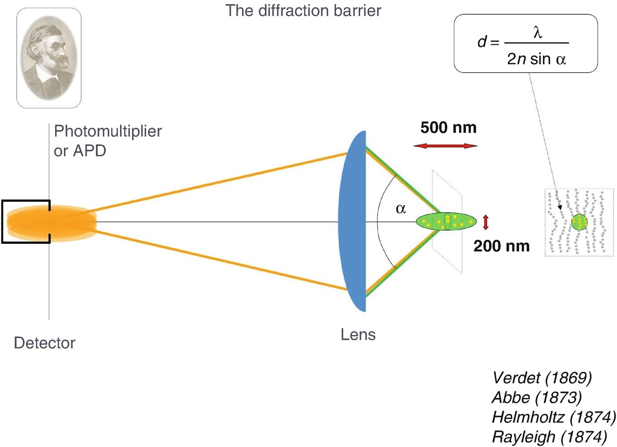
Focusing of light by the microscope (objective) lens cannot occur more tightly than the diffraction (Abbe’s) limit. As a result, all molecules within this diffraction-limited region are illuminated together, emit virtually together, and cannot be told apart. Verdet [2], Abbe [1], Helmholtz [4], Rayleigh [3]
The person who fully appreciated that diffraction poses a serious limit on the resolution was Ernst Abbe, who lived at the end of the nineteenth century and who coined this “diffraction barrier ” in an equation which has been named after him [1]. It says that, in order to be separable, two features of the same kind have to be further apart than the wavelength divided by twice the numerical aperture of the objective lens. One can find this equation in most textbooks of physics or optics, and also in textbooks of biochemistry and molecular biology, due to the enormous relevance of light microscopy in these fields. Abbe’s equation is also found on a memorial which was erected in Jena, Germany, where Ernst Abbe lived and worked, and there it is written in stone. This is what scientists believed throughout the twentieth century. However, not only did they believe it, it also was a fact. For example, if one wanted to look at features of the cellular cytoskeleton in the twentieth century [5], this was the type of resolution obtained.
This equation was coined in 1873. So much new physics emerged during the twentieth century and so many new phenomena were discovered. There should be phenomena—at least one—that could be utilized to overcome the diffraction barrier in a light microscope operating with propagating beams of light and regular lenses. S.W.H. understood that it won’t work just by changing the way the light is propagating, the way the light is focused. [Actually he had looked into that; it led him to the invention of the 4Pi microscope [11, 12], which improved the axial resolution, but did not overcome Abbe’s barrier.] S.W.H. was convinced that a potential solution must have something to do with the major discoveries of the twentieth century: quantum mechanics, molecules, molecular states and so on.
Therefore, he started to check his textbooks again in order to find something that could be used to overcome the diffraction barrier in a light-focusing microscope. In simple terms, the idea was to check out the spectroscopic properties of fluorophores, their state transitions, and so on; maybe there is one that can be used for the purpose of making Abbe’s barrier obsolete . Alternatively, there could be a quantum-optical effect whose potential has not been realized, simply because nobody thought about overcoming the diffraction barrier [13].
With these ideas in mind, one day when he was not very far from [Stockholm] in Åbo/Turku, just across the Gulf of Bothnia, on a Saturday morning, S.W.H. browsed a textbook on quantum optics [14] and stumbled across a page that dealt with stimulated emission. All of a sudden he was electrified. Why?
To reiterate, the problem is that the lens focuses the light in space, but not more tightly than 200 nm. All the features within the 200-nm region are simultaneously flooded with excitation light. This cannot be changed, at least not when using conventional optical lenses. But perhaps we can change the fact that all the features which are flooded with (excitation) light are, in the end, capable of sending light (back) to the detector. If we manage to keep some of the molecules dark—to be precise, put them in a non-signaling state in which they are not able to send light to the detector—we will see only the molecules that can, i.e. those in the bright state. Hence, by registering bright-state molecules as opposed to dark-state molecules , we can tell molecules apart. So the idea was to keep a fraction of the molecules residing in the same diffraction area in a dark state, for the period of time in which the molecules residing in this area are detected. In any case, keep in mind: the state (transition) is the key to making features distinct. And resolution is about discerning features.
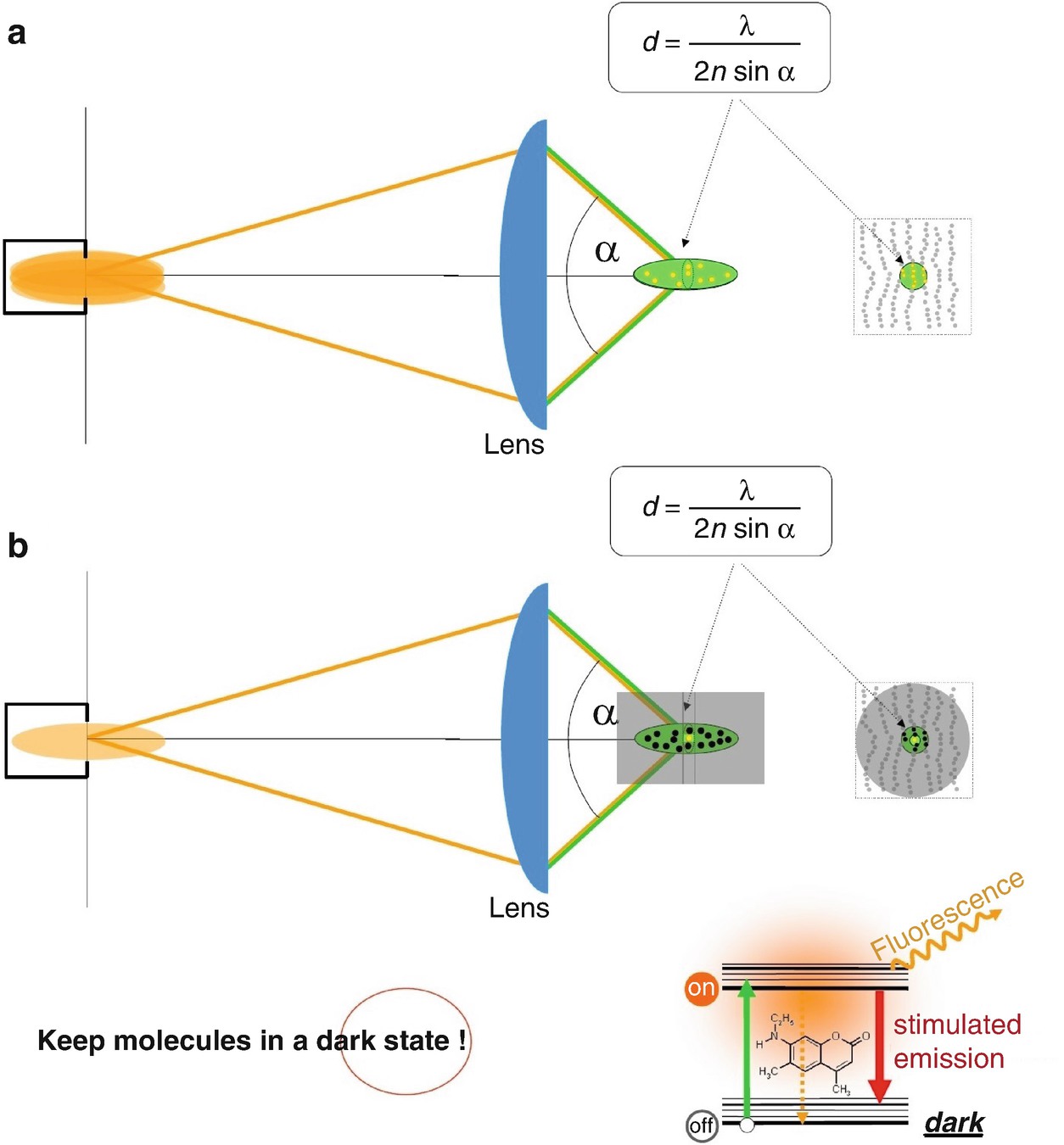
Switching molecules within the diffraction-limited region transiently “off” (i.e. effectively keeping them in a non-signaling state), enables the separate detection of neighbouring molecules residing within the same diffraction region. (a) In fluorescence microscopy operating with conventional lenses (e.g. confocal microscopy ), all molecules within the region covered by the main diffraction maximum of the excitation light are flooded with excitation light simultaneously and emit fluorescence together. This is because they are simultaneously allowed to assume the fluorescent (signalling) state. (b) Keeping most molecules—except the one(s) one aims to register—in a dark state solves the problem. The dark state is a state from which no signal is produced at the detector. Such a transition to the dark “off” state is most simply realized by inducing stimulated emission, which instantaneously forces molecules to their dark (“off”) ground state
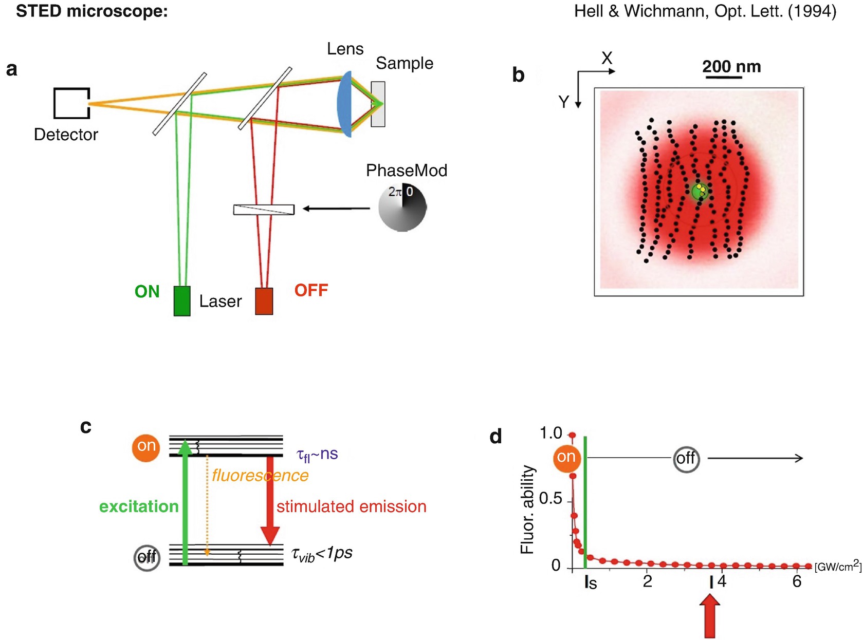
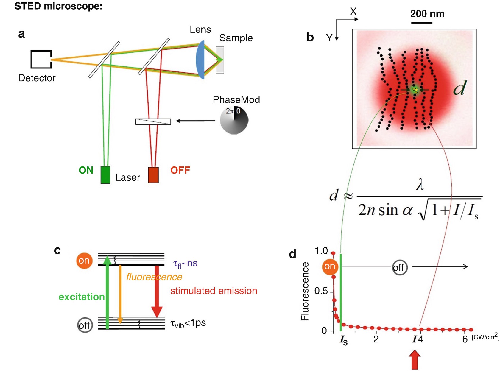
STED microscopy . (a) Setup schematic. (b) Region where the molecule can occupy the “on” state (green) and where it has to occupy the “off” state (red). (c) Molecular transitions. (d) For intensities of the STED light (red) equalling or in excess of the threshold intensity I s, molecules are effectively switched “off”. This is because the STED light will always provide a photon that will stimulate the molecule to instantly assume the ground state, even in the presence of excitation light (green). Thus, the presence of STED light with intensity greater than I s switches the ability of the molecules to fluoresce off. Hell and Wichmann, Opt Lett [15]
The physical condition for achieving this is that the wavelength of the stimulating beam is longer (Fig. 1.3c). The photons of the stimulating beam have a lower energy, so as not to excite molecules but to stimulate the molecules going from the excited state back down to the ground state. There is another condition, however: we have to ensure that there is indeed a red photon at the molecule which pushes the molecule down. We emphasize this because most red-shifted photons pass by the molecules, as there is a finite interaction probability of the photon with a molecule, i.e. a finite cross-section of interaction. But if one applies a stimulating light intensity at or above a certain threshold, one can be sure that there is at least one photon which “kicks” the molecule down to the ground state, thus making it instantly assume the dark state.
Figure 1.3d shows the probability of the molecule to assume the bright state, the S1, in the presence of the red-shifted beam transferring the molecule to the dark ground state. Beyond a certain threshold intensity, I s, the molecule is clearly turned “off”. One can apply basically any intensity of green light. Yet, the molecule will not be able to occupy the bright state and thus not signal. Now the approach is clear: we simply modify this red beam to have a ring shape in the focal plane [19, 24], such that it does not carry any intensity at the centre. Thus, we can turn off the fluorescence ability of the molecules everywhere but at the centre. The ring or “doughnut” becomes weaker and weaker towards the centre, where it is ideally of zero intensity. There, at the centre, we will not be able to turn the molecules off, because there is no STED light, or it is much too weak.
Now let’s have a look at the sample (Fig. 1.3b) and let us assume that we want to see just the fibre in the middle. Therefore, we have to turn off the fibre to its left and the one to its right. What do we do? We cannot make the ring smaller, as it is also limited by diffraction. Abbe would say: “Making narrower rings of light is not possible due to diffraction.” But we do not have to do that. Rather, we simply have to “shut off” the molecules of the fibres that we do not want to see, that is, we make their molecules dwell in a dark state, until we have recorded the signal from that area. Obviously, the key lies in the preparation of the states. So what do we do? We make the beam strong enough so that the molecules even very close to the centre of the ring are turned “off” because they are effectively confined to the ground state all the time. This is because, even close to the centre of the ring, the intensity is beyond the threshold I s in absolute terms.
Now we succeed in separation: only in the position of the doughnut centre are the molecules allowed to emit, and we can therefore separate this signal from the signal of the neighbouring fibres. And now we can acquire images with subdiffraction resolution : we can move the beams across the specimen and separate each fibre from the other, because their molecules are forced to emit at different points in time. We play an “on/off game”. Within the much wider excitation region, only a subset of molecules that are at the centre of the doughnut ring are allowed to emit at any given point in time. All the others around them are effectively kept in the dark ground state. Whenever one makes a check which state they are in, one will nearly always find those molecules in the ground state.

Nuclear pore complex architecture in an intact cell nucleus imaged by (a) confocal microscopy (diffraction-limited), and (b) STED nanoscopy. The data was published in [25]
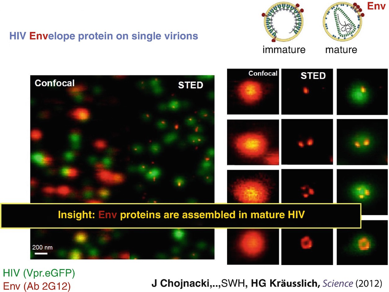
STED nanoscopy of the HIV Envelope protein Env on single virions. Confocal microscopy is not able to reveal the nanoscale spatial distribution of the Env proteins; the images of the Env proteins on the virus particles look like 250–350 nm sized blurred spots (orange, left column). STED microscopy reveals that the Env proteins form spatial patterns (center column, orange), with mature particles having their Env strongly concentrated in space (panel in top row of center column, orange). The data was published in [26]
Of course, a strength of light microscopy is that we can image living cells by video-rate recording with STED microscopy. An example are synaptic vesicles in the axon of a living neuron [20]. One can directly see how they move about and we can study their dynamics and their fate over time. It is clearly important to be able to image living cells.
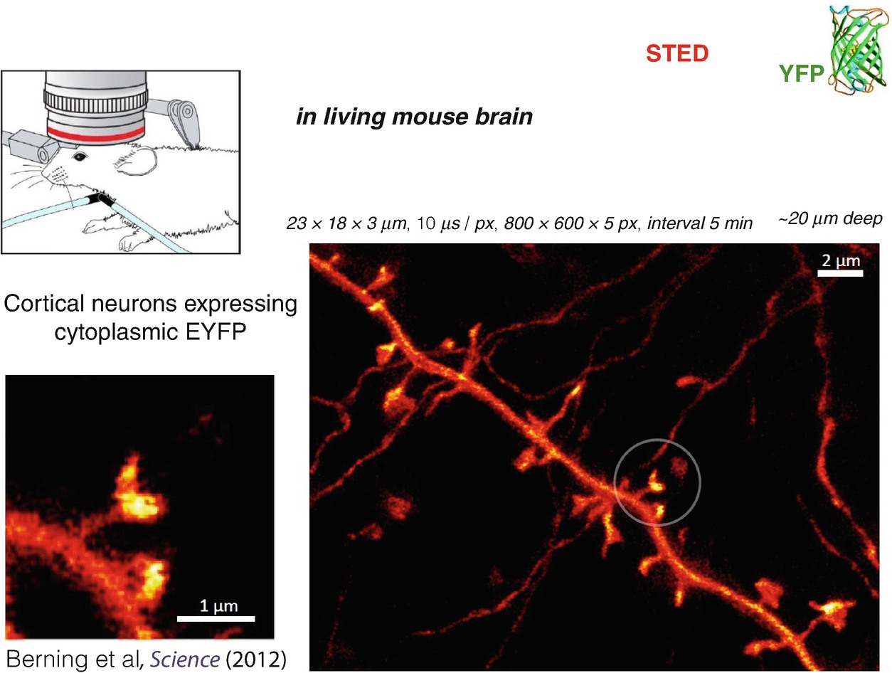
STED nanoscopy in living mouse brain. The recording shows a part of a dendrite of a neuron expressing a yellow fluorescent protein (EYFP) in the cytosol, thus highlighting the neuron amidst surrounding (non-labelled) brain tissue. The three to fourfold improved resolution over confocal and multiphoton excitation fluorescence microscopy reveals the dendritic spines (encircled) with superior clarity, particularly the cup-like shape of some of their terminals containing the receiving side of the synapses. The data was published in [21]
(a–d) Resolution scaling in the STED/RESOLFT concepts: an extension of Abbe’s equation . The resolution scales inversely with the square-root of the ratio between the maximum intensity at the doughnut crest and the fluorophore-characteristic threshold intensity I s
In the situation depicted in Fig. 1.7b, we cannot separate two of the close-by molecules because both are allowed to emit at the same time. But let us make the beam a bit stronger, so that only one molecule “fits in” the region in which the molecules are allowed to be “on”. Now the resolution limit is apparent: it is the size of a molecule, because a molecule is the smallest entity one can separate. After all, we separate features by preparing their molecules in two different states, and so it must be the molecule which is the limit of spatial resolution. When two molecules come very close together, we can separate them because at the time one of them is emitting, the other one is “off” and vice versa [28, 30–32].
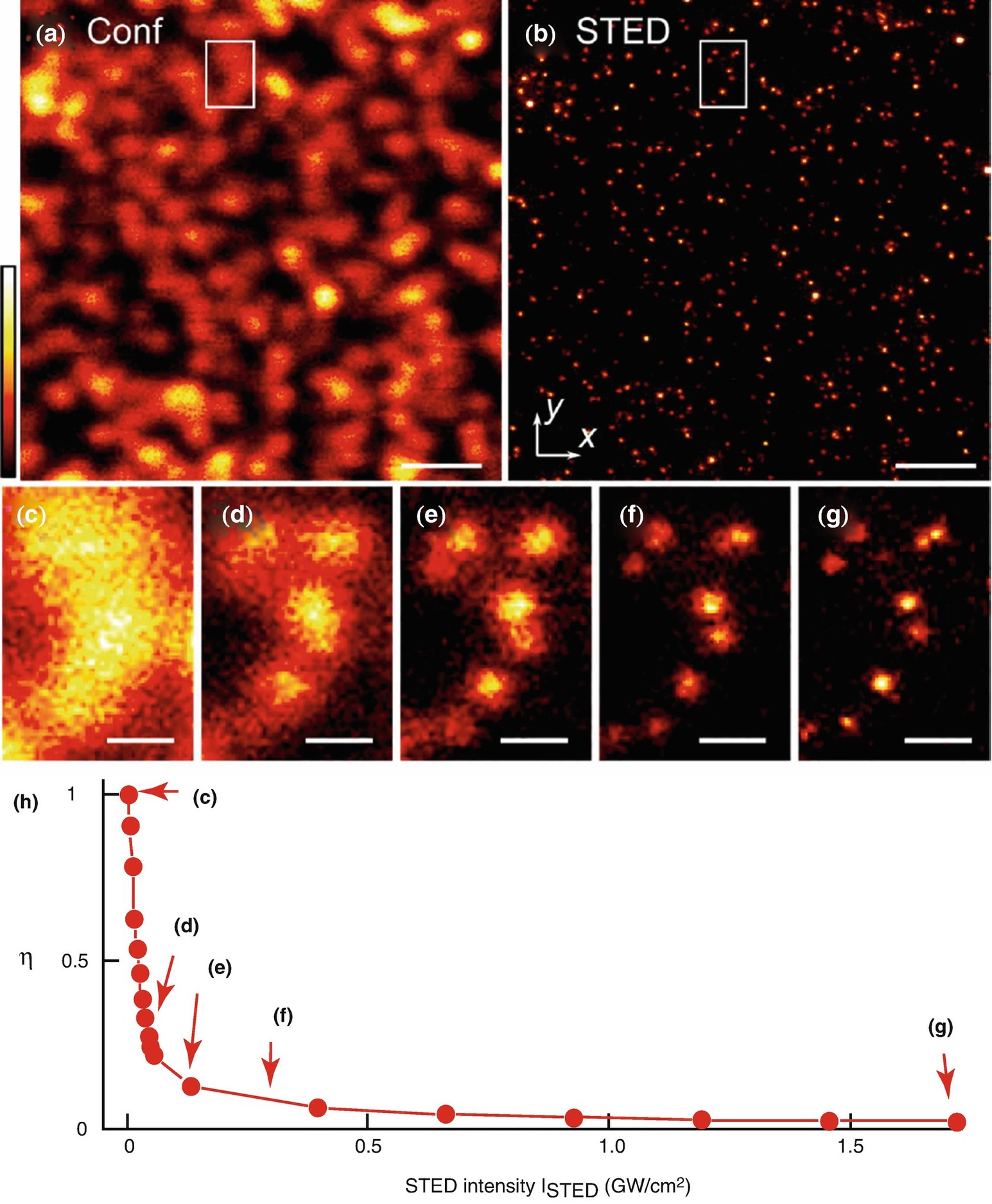
Tunable resolution enhancement realized by STED microscopy . (a, b) Confocal (a) and STED (b) image of fluorescent beads with average size of ~24 nm on a cover slip. (c–g) The area of the white rectangle shown in (a) and (b) recorded with different STED intensities. The resolution gain can be directly appreciated. (h) STED depletion η vs. STED-light intensity measured on the same sample. The intensity settings for the measurements (c–g) are marked by red arrows. Scale bars 1 μm (a, b), 200 nm (c–g). Reproduced with permission from [33]
Does one typically obtain molecular spatial resolution, and what about in a cell? For STED microscopy right now, the standard of resolution is between 20 and 40 nm depending on the fluorophore, and depending on the fluorophore’s chemical environment [25]. But this is something which is progressing; it is under continuous development. With fluorophores which have close-to-ideal properties and can be turned “on” and “off” as many times as desired, we can do much better, of course.
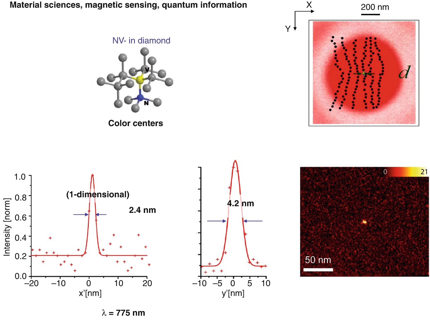
Fluorophores affording virtually unlimited repetitions of the resolution-enabling on-off state transitions provide the present resolution records in far-field optical imaging using STED, in the single-digit nanometer regime. Color centers (charged nitrogen vacancy centers) in diamond hold great potential for various other applications, notably in magnetic sensing and quantum information, which may be eventually read out with diffraction-unlimited spatial resolution using conventional lenses, i.e. even when packed very densely at the nanometer scale
This may look like a proof-of-principle experiment, and to some extent it is. But it is not just that, there is another reason to perform these experiments [34, 36, 37]. The so-called charged nitrogen vacancies are currently regarded as attractive candidates for quantum computation: as qubits operating at room temperature [38, 39]. They possess a spin state with a very long coherence time and which can be prepared and read out optically. Being less than a nanometer in size, they can sense magnetic fields at the nanoscale [40, 41]. There inherently are nanosensors in there, and STED is perhaps the best way of reading out the state and the magnetic fields at the nanoscale. In the end, this could make STED an interesting candidate perhaps for reading out qubits in a quantum computer, or who knows … Development goes on!
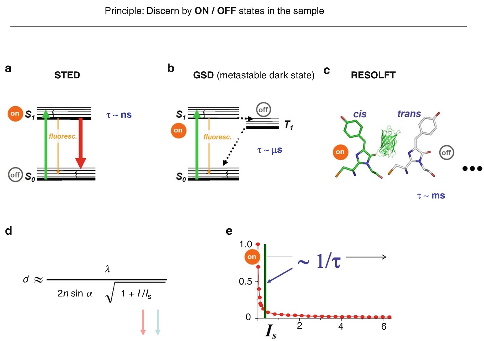
States and state transitions utilized in (a) STED, (b) GSD and (c) RESOLFT nanoscopy . (d) The intensity I s for guaranteeing the transition from the on- to the off-state is inversely related to the state lifetime. The longer the lifetime of the involved states, the fewer photons per second are needed to establish the on-off state difference which is required to separate features residing within the diffraction barrier
Indeed, it turns out that there is a strong reason for looking into other types of states and state transitions. Consider the state lifetimes (Fig. 1.10). For the basic STED transition, the lifetime of the state, the excited state, is nanoseconds (Fig. 1.10a). For metastable dark states used in methods termed ground state depletion (GSD) microscopy [42–44] (Fig. 1.10b) the lifetime of the state is microseconds, and for isomerization it is on the order of milliseconds (Fig. 1.10c). Why are these major increases in the utilized state lifetime relevant?
Well, just remember that we separate adjacent features by transferring their fluorescent molecules into two different states. But if the state—one of the states—disappears after a nanosecond, then the difference in states created disappears after a nanosecond. Consequently, one has to hurry up putting in the photons, creating this difference in states, as well as reading it out, before it disappears. But if one has more time—microseconds, milliseconds—one can turn molecules off, read the remaining ones out, turn on, turn off ….; they stay there, because their states are long-lived. One does not have to hurry up putting in the light, and this makes this “separation by states ” operational at much lower light levels [28, 42].
To be more formal, the aforementioned intensity threshold Is scales inversely with the lifetime of the states involved (Fig. 1.10e): the longer the lifetime, the smaller is the Is, and the diffraction barrier can be broken using this type of transition at much lower light levels. Is goes down from megawatts (STED), kilowatts (GSD) down to watts per square centimetre for millisecond switching times—a six orders of magnitude range [28]. This makes transitions between long-lived states very interesting, of course. Here in the equation (Fig. 1.10d), Is goes down and with that of course also I goes down because one does not need as many photons per second in order to achieve the same resolution d.

Parallelization of the STED/RESOLFT concept holds the key to faster imaging. The diffraction problem has to be addressed only for molecules residing within a diffraction-limited region. Thus, many intensity minima (‘doughnuts’) are produced, at mutual distances greater than the diffraction limit, for highly efficient scanning of large sample areas. The use of highly parallelized schemes is greatly facilitated by harnessing transitions between long-lived molecular on-off states, such as cis/trans

Massively parallelized RESOLFT nanoscopy. Here, an array of ~114,000 intensity minima (zeros) was used to image a living cell in 2 s. The data was published in [48]
Notwithstanding the somewhat different optical arrangement, the key is the molecular transition. Selecting the right molecular transition determines the parameters of imaging. The imaging performance, including the resolution and the contrast level, as well as other factors, is actually determined by the molecular transition chosen [32].
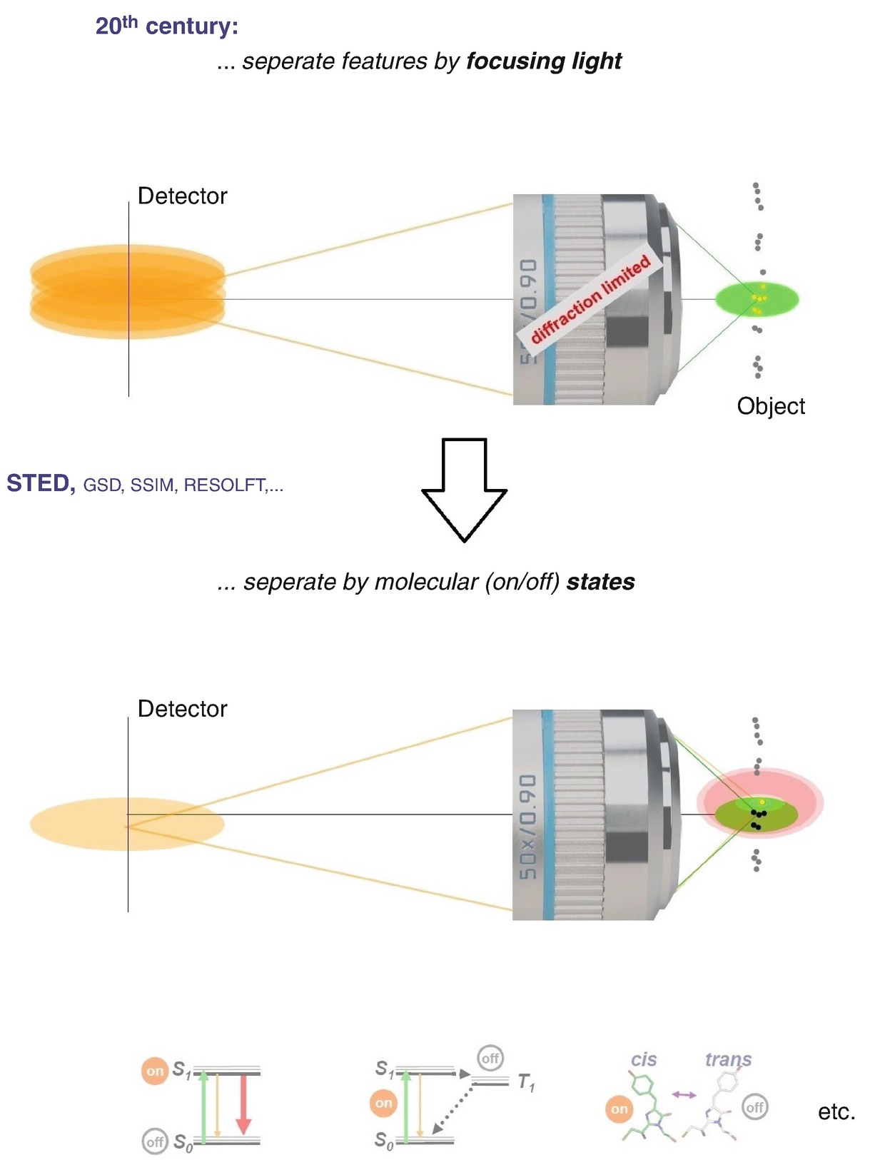
Paradigm shift in the use of the physical phenomenon by which features are discerned in a far-field optical (fluorescence) microscope: from focusing of light, which is inherently diffraction-limited, to using a molecular state transition, such as a transition between an “on” and an “off” state, which is not
Do not separate just by focusing. Separate by molecular states, in the easiest case by “on/off”-states [28–31]. If separating by molecular states, one can indeed distinguish the features, one can tell the molecules apart even though they reside within the region dictated by diffraction. We can tell, for instance, one molecule apart from its neighbours and discern it (Fig. 1.13, bottom). For this purpose, we have our choice of states that I have introduced already (Fig. 1.10) which we can use to distinguish features within the diffraction region.
In the methods described, STED, RESOLFT and so on, the position of the state—where the molecule is “on”, where the molecule is “off”—is determined by a pattern of light featuring one or more intensity zeros, for example a doughnut. This light pattern clearly determines where the molecule has to be “on” and where it has to be “off”. The coordinates X, Y, Z are tightly controlled by the incident pattern of light and the position(s) of its zero(s). Moving the pattern to the next position X, Y, Z—one knows the position of the occurrence of the “on” and “off” states already. One does not necessarily require many detected photons from the “on” state molecules, because the detected photons are merely indicators of the presence of a feature. The occurrence of the state and its location is fully determined by the incident light pattern.
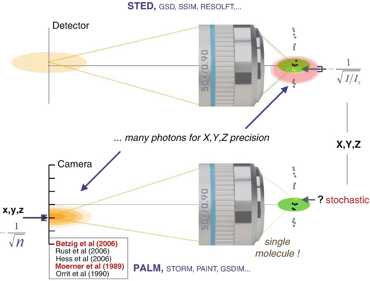
Both in coordinate-targeted and in coordinate-stochastic nanoscopy methods , many photons are required to define or establish, respectively, molecular coordinates at subdiffraction scales. In the coordinate-targeted mode (STED, RESOLFT, etc.), the coordinates of (e.g.) the “on”-state are established by illuminating the sample with a pattern of light featuring an intensity zero; the location of the zero and the pattern intensity define the coordinates with subdiffraction precision. In the coordinate-stochastic mode (PALM, STORM etc.), the coordinates of the randomly emerging “on”-state molecules are established by analysing the light patterns emitted by the molecules (localization). Precision of the spatial coordinates increases in both cases with the number of photons in the patterns of the spatial coordinates, i.e. by the intensity of the pattern. In both families of methods, neighbouring molecules are discerned by transiently creating different molecular states in the sample. The references shown are to [8, 9, 49, 51, 52] described in the text
An interesting insight here is that one needs a bright pattern of emitted light to find out the position just as one needs a bright pattern of incident light in STED/RESOLFT to determine the position of emission. Not surprisingly, one always needs bright patterns of light when it comes to positions, because if one has just a single photon, this alone tells nothing. The photon can go anywhere within the realm of diffraction, there is no way to control where it goes within the diffraction zone. In other words, when dealing with positions, one needs many photons by definition, because this is inherent to diffraction. Many photons are required for defining positions of “on”- and “off”-state-molecules in STED/RESOLFT microscopy, just as many photons are required to find out the position of “on”-state molecules in the stochastic method PALM.

To parallelize STED/RESOLFT scanning, a “widefield” arrangement with an array of intensity minima (e.g. an array of doughnuts) may be used. The numbers of molecules at these readout target coordinates do not matter, while PALM requires that there may be only a single “on”-state molecule within a diffraction zone, i.e. within the distance dictated by the diffraction barrier. [More precisely: the number of molecules per diffraction zone has to be so low that each molecule is recognized individually.] The position of each on-state molecule is however completely random in space. I s can be regarded as the number of photons that one needs to ensure that there is at least one photon interacting with the molecule, pushing it from one state to the other in order to create the required difference in molecular states. I/I s is, so to speak, the number of photons which really elicit the (on/off) state transition at the molecule, while most of the others just “pass by”. Similarly, in the PALM concept, the number of photons n in 1/√(n) is the number of those photons that are really detected at the coordinate-giving pixelated detector (camera), i.e. that really contribute to revealing the position of the emitting molecule. In other words, in both concepts, to attain a high coordinate precision, one needs many photons that act. The references shown are to [8, 9, 49, 51, 52] described in the text
Although the PALM principle can also be implemented on a single diffraction zone only (i.e. using a single focused beam of light), it is usually implemented in a “parallelized” way, i.e. on a larger field of view containing many diffraction zones. PALM parallelization requires that there may be only a single “on”-state molecule within a diffraction zone, i.e. within the distance dictated by the diffraction barrier. However, the position of this molecule is completely random. Therefore, we have to make sure that the “on”-state molecules are far enough apart from each other, so that they are still identifiable as separate molecules. While in (STED/RESOLFT) the position of a certain state is given by the pattern of light falling on the sample, position in PALM is established from the pattern of (fluorescence) light coming out of the sample.
What does I/I s in STED/RESOLFT stand for? I s can be seen as the number of photons that one needs to ensure that there is at least one photon interacting with the molecule, pushing it from one state to the other in order to create the required difference in molecular states. I/I s is, so to speak, the number of photons which really “can do something” at the molecule while most of the others just “pass by”. Similarly, in the PALM concept, the number of photons n in 1/√(n) is the number of those photons that are detected, i.e. that really contribute to revealing the position of the emitting molecule. In other words, in both concepts, to attain a high coordinate precision, one needs many photons that really do something. This analogy very clearly shows the importance of the number photons to achieve coordinate precision in both concepts.
However, in both cases the separation of features is, of course, accomplished by an “on/off”-transition [28–31]. This is how we make features distinct, how we tell them apart. As a matter of fact, all the super-resolution methods which are in place right now and really useful, achieve molecular distinguishability by transiently placing the molecules that are closer together than the diffraction barrier in two different states for the time period in which they are jointly scrutinized by the detector. “Fluorescent” and “non-fluorescent” is the easiest pair of states to play with, and so this is what has worked out so far.

3D STED microscopy for simultaneously increasing the resolution in the focal plane and along the optic axis. (Left Top) Schematic setup . The STED power is distributed between the two phase plates (Plat and P3D) by using a combination of a λ/2 plate and a polarizing beam splitter (PBS) . The second PBS recombines the two beams incoherently. The excitation (Exc) and STED beams are overlaid by a dichroic mirror (DM). A λ/4 plate ensures the circular polarization of all beams prior to being focused by the objective lens (OL). The fluorescence signal (Fl) is collected by the same lens. (Left Bottom) Focal intensity distributions of excitation and STED beams measured using gold beads in reflectance mode. From left to right: Excitation, STED beam from Plat arm resulting in the focal deexcitation pattern STEDlat, STED beam from P3D arm yielding STED3D, incoherent combination of both arms (30% STEDlat/70% STED3D power distribution). The latter distribution results in an efficient coverage of the volume around the focal point. Scale bars 500 nm. (Right) (a–d) 3D nanoscale image of dilute distribution of 20 nm diameter fluorescent spheres on glass. xy sections of (a) confocal and (b) STED. (c) Confocal and (d) STED xz sections along the dashed blue line indicated in panels (a) and (b). Individual beads can be easily resolved in the STED images. Comparing panel (c) with panel (d), note the significant reduction in cross-sectional area in the STED xz-image (e, f) Intensity profile along the (e) x and (f) z direction for sections indicated by the white arrows in panels (c) and (d). All presented data is raw data. (g) Focal volume reduction relative to confocal focal volume measured using 20 nm fluorescent spheres. The combination of two de-excitation patterns gives a maximal volume reduction factor of 125. Scale bars 1 μm. From [54], reproduced with permission

isoSTED: Fluorescence microscopy setup with isotropic 3D focal spot. (a) Beams for excitation, STEDxy (lateral) and STEDz (axial) are combined using a dichroic mirror (DCSP) and then fed through a beam scanner into a 4Pi unit with two opposing objective lenses (O1 and O2; HCX PL APO 100x, 1.46 NA OIL CORR). The fluorescence light (orange) collected by both lenses backpropagates along the same optical path to the detector, passing through the DCSP and a second dichroic mirror (DCLP) . The pivot plane (PP) of all scanning beams is conjugated to the entrance pupils of the objective lenses. The incoming beams are divided by a polarizing beam-splitter (PBS) and coherently superimposed at both lenses’ common focal plane inside the sample (S). A piezo-driven mirror (MP) controls the difference in pathlength between both cavity arms and thereby the 4Pi phases of all beams. The polarization state of STEDxy and STEDz is adjusted by two half-wave retarder plates (H1 and H2). The excitation beam and the STED beams for lateral (STEDxy, imprinted with a circular phase ramp (PM)) and axial (STEDz) fluorescent spot compression are polarized under α = 45° with respect to the perpendicular direction (n) to the splitting plane (p) of the polarizing beam-splitter. STEDxy and STEDz are polarized orthogonal to each other. (b) Calculated focal intensity distributions and formation of the STED PSF with respective wavelengths, λ, and 4Pi phases ϕ. (c) Isotropic effective focal spot (PSF) on the nanoscale. (Left) Calculated PSF of a confocal fluorescence microscope and the corresponding spherical PSF of the isoSTED microscope at Im/Is = 15 (NA = 1.4). (Middle) Experimental counterpart to (left) as measured with a 21-nm-diameter fluorescence bead. The FWHM of the confocal setup (1.46 NA) is 165 nm in the lateral and 405 nm in the axial direction. Switching on the STED pattern shown in b leads to a largely spherical main focal fluorescence spot. (Right) Gaussian fits through the lateral and axial profiles of the focal spot yield indicated FWHM, corresponding to an isotropic far-field optical 3D resolution of λ/16. Baselines are marked with colored circles. Scale bars, 250 nm. From [55], reproduced with permission
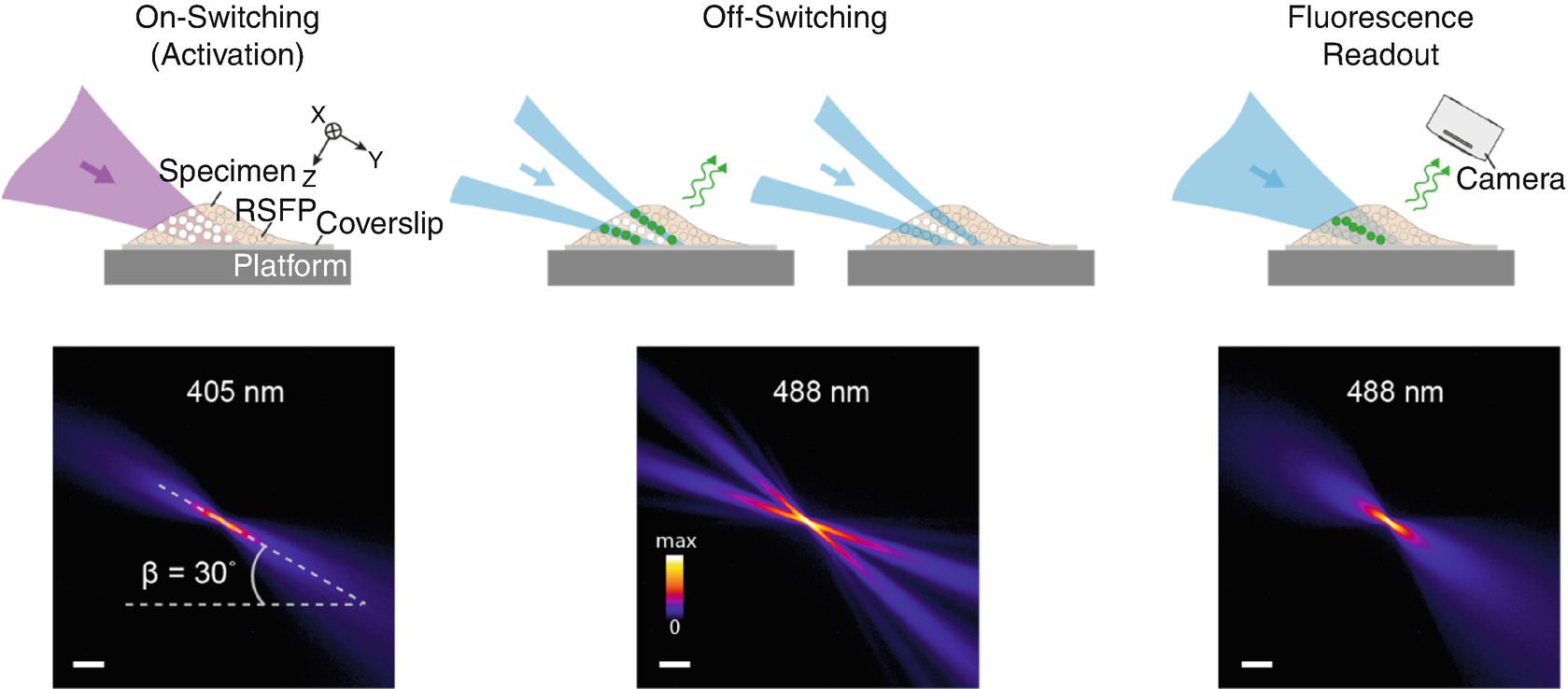
Lightsheet (LS)-RESOLFT concept . A living specimen expressing RSFPs is grown on a coverslip mounted on a movable platform. The specimen is illuminated (here in y direction) perpendicular to the detection axis (z). Only in a thin diffraction-limited section, RSFPs are switched from their initial off state (unfilled dots) to the on state (white dots) by an activating LS. None of the fluorophores outside the illuminated volume is affected by the laser light. An LS featuring a central zero-intensity plane switches off the activated RSFPs above and below the detection focal plane (x–y). For negative-switching RSFPs, this is a competing process to fluorescence (green dots and arrows). For off-switching light intensities above the threshold of the RSFPs, only fluorophores within a slice of subdiffraction thickness remain activated. These can be read out by a third LS and contribute to the LS-RESOLFT image. The platform is displaced to the next position in the scanning sequence for another illumination cycle. The lower row shows measured y–z cross-sections of the applied LSs visualized in fluorescent medium. The sheets impinge on the coverslip at an angle of 30°. (Scale bar, 100 μm.) From [57], reproduced with permission

Super-resolution microscopy in vivo: mouse and fruit fly nanoscopy. (a) STED nanoscopy of a mouse with enhanced yellow fluorescent protein-labelled neurons. Shown are dendritic and axonal details in the molecular layer of the somatosensory cortex of a living, anesthetized mouse. Optical access to the brain cortex was enabled by a cover glass-sealed cranial window. Top panel: image of a neuron. Bottom panel: STED time-lapse recording of spine morphology dynamics. Scale bars: 1 μm. (b) STED imaging of synaptic protein distribution. Example: PSD95, the abundant scaffold protein at the postsynaptic membrane, which organizes numerous other synaptic proteins. (Left) The cartoons show the in-vivo labeling of endogenous PSD95-HaloTag , a self-labeling enzymatic protein tag, with organic fluorophores. (Right) Depending on the orientation of the individual spine head imaged with respect to the focal plane, the intricate spatial organization of PSD95 at the synapse is revealed in the STED mode. Scale bars: 500 nm. (c) RESOLFT imaging of the microtubule cytoskeleton of intact, living Drosophila melanogaster larvae. A second instar larva ubiquitously expressing a fusion protein composed of the reversibly switchable fluorescent protein (RSFP) rsEGFP2 fused to α-tubulin was placed under a coverslip and imaged through the intact cuticle. Left: confocal overview. Middle and right: magnifications of the area indicated by the corresponding square. Shown are comparisons of confocal and RESOLFT recordings (separated by a dashed line), exemplifying the difference in resolution. Scale bars: 10 μm, 1 μm and 500 nm (from left to right). Part (a) is adapted from [21]. Reprinted with permission from AAAS. Part (c) is adapted with permission from [63], CC-BY 3.0. Parts (a) and (c) reproduced with permission from [64], part (b) from [65]
1.2 Recent Developments: Nanoscopy at the MINimum

Concepts with improved sample-responsive implementation of the on-off switching. (a) The MINFIELD concept: Lower local de-excitation intensities in STED nanoscopy for image sizes below the diffraction limit. (Left) In STED imaging with pulsed lasers, the ability of a fluorophore to emit fluorescence decreases nearly exponentially with the intensity of the beam de-exciting the fluorophore by stimulated emission. Is can be defined as the intensity at which the fluorescence signal is reduced by 50%. Fluorophores delivering higher signal are defined as on, whereas those with smaller signal are defined as off. (Middle) The STED beam is shaped to exhibit a central intensity zero in the focal region (i.e., a doughnut), so that (Right) molecules can show fluorescence only if they are located in a small area in the doughnut center. This area decreases with increasing total doughnut intensity. Due to its diffraction-limited nature, the intensity distribution of the STED focal beam extends over more than half of the STED-beam wavelength and exhibits strong intensity maxima, significantly contributing to photobleaching. By reducing the size of the image field to an area below the diffraction limit, where the STED beam intensity is more moderate (i.e., around the doughnut minimum; compare image area indicated in the Middle), one can reduce the irradiation intensities in the area of interest, inducing lower photobleaching and allowing the acquisition of more fluorescence signal at higher resolution. Scale bar: 200 nm. (b) DyMIN (Dynamic Intensity MINimum ) STED imaging. (Left) Concept illustrated for two fluorophores spaced less than the diffraction limit. Signal is probed at each position, starting with a diffraction-limited probing step (PSTED = 0, Top), followed by probing at higher resolution (PSTED > 0). At any step, if no signal indicates the presence of a fluorophore, the scan advances to the next position without applying more STED light to probe at higher resolution. For signal above a threshold (e.g., T1, Upper Middle), the resolution is increased in steps (Lower Middle), with decisions taken based on the presence of signal. This is continued up to a final step of Pmax (full resolution where required). For the highest-resolution steps, directly at the fluorophore(s), the probed region itself is located at the minimum of the STED intensity profile (Bottom). (c) Dual-color isotropic nanoscopy of nuclear pore components and lamina with DyMIN STED: Confocal and 3D DyMIN STED recordings of nuclear pore complexes (shown in green) and lamina (red). Scale bars: 500 nm. (d) DyMIN STED imaging of DNA origami structures with fluorophore assemblies. The DNA origami-based nanorulers with nominally 30-nm separation (10-nm gap) consisted of two groups of ~15 ATTO647N fluorophores, on average, each. Accounting for the known ~20-nm extent of the fluorophore groups (compare schematic), the widths of the Gaussians imply an effective PSF of ~17 nm (FWHM). Scale bars: 200 nm. Figures reproduced with permission from [67] (a) and [68] (b–d)
DyMIN is a related recording strategy [68] which minimizes exposure to unduly high intensities except at scanning steps where these intensities are strictly required for resolving features (Fig. 1.20b–d). Like MINFIELD, the DyMIN approach achieves dose reductions by up to orders of magnitude, particularly for relatively sparse fluorophore distributions . Initially demonstrated for STED immunofluorescence imaging, both MINFIELD and DyMIN will be explored for other classes of fluorophores, including the inherently lower-light-level RESOLFT nanoscopy variants with genetically encoded fluorescent proteins. The recently described organic switchable photochromic compounds [70] will also be further developed as attractive alternatives in this regard. The synergistic combination of two separate fluorophore state transitions in a recent concept termed multiple off-state transitions (MOST) for nanoscopy [66] has also enabled many more image frames to be captured, at much improved contrasts and with lower STED light dose at a given resolution than for standard STED. Approaches to directly count molecules with STED have also been developed [71], and can be used to quantify the composition of suitably labeled molecular clusters.

Principles of MINFLUX, a concept for localizing photon emitters in space, illustrated in a single dimension (x) by using a standing light wave of wavelength λ. (a) The unknown position x
m of a fluorescent molecule is determined by translating the standing wave, such that one of its intensity zeros travels from x = −L/2 to L/2, with x
m somewhere in between. (b) Because the molecular fluorescence f(x) becomes zero at x
m, solving f(x
m) = 0 yields the molecular position x
m. Equivalently, the emitter can also be located by exposing the molecules to only two intensity values belonging to functions I
0(x) and I
1(x) that are fixed in space having zeros at x = −L/2 and L/2, respectively. Establishing the emitter position can be performed in parallel with another zero, by targeting molecules further away than λ/2 from the first one. (c) Localization considering the statistics of fluorescence photon detection: Success probability p
0(x) for various beam separations L are shown as listed in the legend for λ = 640 nm. The fluorescence photon detection distribution P(n
0|N = n
0 + n
1 = 100) conditioned to a total of 100 photons is plotted along the right vertical axis of normalized detections n
0/N for each L. The distribution of detections is mapped into the position axis x through the corresponding p
0(x,L) function (gray arrows), delivering the localization distribution P( |N = 100). The position estimator distribution contracts as the distance L is reduced. (d) Cramér-Rao bound (CRB)
for each L. Precision is maximal halfway between the two points where the zeros are placed. For L = 50 nm, detecting just 100 photons yields a precision of 1.3 nm. Figure reproduced from [72]. Reprinted with permission from AAAS
|N = 100). The position estimator distribution contracts as the distance L is reduced. (d) Cramér-Rao bound (CRB)
for each L. Precision is maximal halfway between the two points where the zeros are placed. For L = 50 nm, detecting just 100 photons yields a precision of 1.3 nm. Figure reproduced from [72]. Reprinted with permission from AAAS
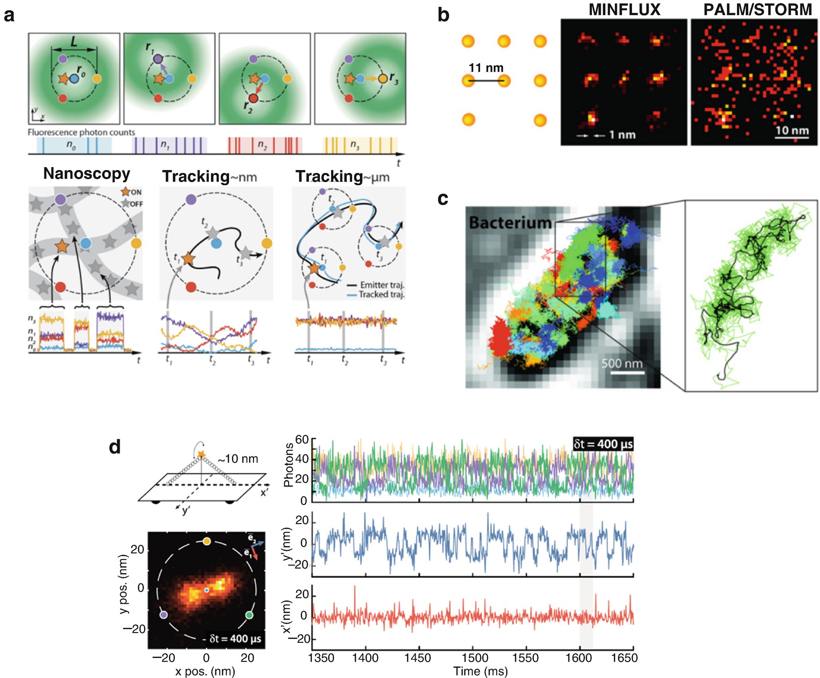
The MINFLUX concept: molecular resolution in fluorescence nanoscopy. (a) Implementation of MINFLUX in 2D fluorescence imaging and tracking. (Top) Diagrams of the positions of the doughnut in the focal plane and resulting fluorescence photon counts. (Bottom) Basic application modalities of MINFLUX. (Left) Nanoscopy: A nanoscale object features molecules whose fluorescence can be switched on and off, such that only one of the molecules is on within the detection range. They are distinguished by abrupt changes in the ratios between the different n 0,1,2,3 or by intermissions in emission. (Middle) Nanometer-scale (short-range) tracking: The same procedure can be applied to a single emitter that moves within the localization region of size L. As the emitter moves, different fluorescence ratios are observed that allow the localization. (Right) Micron-scale (long-range) tracking: If the emitter leaves the initial L-sized field of view, the triangular set of positions of the doughnut zeros is (iteratively) displaced to the last estimated position of the molecule. By keeping it around r 0 by means of a feedback loop, photon emission is expected to be minimal for n 0 and balanced between n 1, n 2, and n 3, as shown. (b) With MINFLUX nanoscopy one can, for the first time, separate molecules optically which are only a few nanometers apart from each other. On the left, a schematic of the molecules is presented. Whereas the ultra-high resolution PALM/STORM microscopy at the same molecular brightness (Right) delivers a diffuse image of the molecules (here in a simulation under ideal technical conditions), the position of the individual molecules can be easily discerned with the practically realized MINFLUX (middle). (c) Many much faster movements can be followed than is possible with STED or PALM/STORM microscopy. Left: Movement pattern of 30S ribosomes (colored) in an E. coli bacterium (gray scale). Right: Movement pattern of a single 30S ribosome (green) shown enlarged. (d) MINFLUX tracking of rapid movements of a custom-designed DNA origami. (Top left) Diagram of the DNA origami construct with a single ATTO 647N fluorophore attached at the center of the bridge (10 nm from the origami base). By design, the emitter can move on a half-circle above the origami and is thus ideally restricted to a 1D movement. (Bottom left) Histogram of 6118 localizations of the sample with δt = 400 μs time resolution and a 1.5 × 1.5-nm binning. The predominant motion is along a single direction. (Right, Upper) A 300-ms excerpt of the photon count trace (time resolution δt = 400 μs per localization). The color coding corresponds to the zero positions shown to the left. (Right, Lower) Mean-subtracted trajectory. Figure reproduced from [72] (a) (reprinted with permission from AAAS) and [73] (d)
While the experimental developments of the MINFLUX concept are still in the beginnings, it is worth commenting on the fundamental advantage over localization based on the emitted fluorescence alone. As discussed in [72, 73], in PALM/STORM, as in camera-based tracking applications, a molecule’s position is inferred from the maximum of its fluorescence diffraction pattern (back-projected into sample space). The precision of such camera-based localization ideally reaches σcam ≥ σPSF/√N, with σPSF being the standard deviation of the pattern and N the number of fluorescence photons making up the pattern [74]. Note that σcam is thus clearly bounded by the finite fluorescence emission rate, which for currently used fluorophores rarely allows more than a few hundred photon detections per millisecond (<1 MHz). Moreover, emission is frequently interrupted and eventually ceases due to blinking and bleaching. This also keeps the photon emission rate as the limiting factor for the obtainable spatio-temporal resolution. As a result, state-of-the-art single-molecule tracking performance long remained in the tens of nanometer per several tens of millisecond range. Drawing on the basic ideas of the coordinate determination employed in STED/RESOLFT microscopy, the MINFLUX concept addresses these fundamental limitations [72]. By localizing individual emitters with an excitation beam featuring an intensity minimum that is spatially precisely controlled, MINFLUX takes advantage of coordinate targeting for single-molecule localization. The basic steps are illustrated for one spatial dimension in Fig. 1.21. In a typical two-dimensional MINFLUX implementation, the position of a molecule is obtained by placing the minimum of a doughnut-shaped excitation beam at a known set of spatial coordinates in the molecule’s proximity. These coordinates are within a range L in which the molecule is anticipated (Fig. 1.22a). Probing the number of detected photons for each doughnut minimum coordinate yields the molecular position. It is the position at which the doughnut would produce minimal emission, if the excitation intensity minimum were targeted to it directly. As the intensity minimum is ideally a zero, it is the point at which emission is ideally absent. The precision of the position estimate increases with the square root of the total number of detected photons and, more importantly, by decreasing the range L, the spatial scale inserted from the outside into the experiment. For small ranges L for which the intensity minimum is approximated by a quadratic function, the localization precision does not depend on any wavelength and, for the case of no background and perfect doughnut control, the precision σMINFLUX simply scales with L/√N at the center of the investigated range. In other words, the better the coordinates of the excitation minimum match the position of the molecule, the fewer fluorescence detections are needed to reach a given precision. In the conceptual limit where the excitation minimum coincides with the position of the emitter, i.e. L = 0, the emitter position is rendered by vanishing fluorescence detection. This is contrary to conventional centroid-based localization where precision improvements are tightly bound to having increasingly larger numbers of detected photons.
The already demonstrated tracking of fluorophores with substantially sub-millisecond position sampling (Fig. 1.22c) is only the beginning in a quest for highest spatiotemporal capabilities (compare data in Fig. 1.22d) [73]. The inherent confocality should also provide a critical advantage when considering imaging in more dense and three-dimensional specimens, such as brain slices and in-vivo imaging scenarios. With further development of other aspects, including field-of-view enlargement, etc., MINFLUX is bound to transform the limits of what can be observed in cells and molecular assemblies with light. This should most probably impact cell and neurobiology and possibly also structural biology. Moreover, it should be a great tool for studying molecular interactions and intra-macromolecular dynamics in a range that has not been accessible so far.
Acknowledgements
Substantial portions of the discussion in this chapter have been only slightly modified from the published text of the Nobel Lecture, as delivered by Stefan W. Hell in Stockholm on December 8, 2014 (Copyright The Nobel Foundation, which has granted permission for reuse of the materials.)

Open Access This chapter is licensed under the terms of the Creative Commons Attribution 4.0 International License (http://creativecommons.org/licenses/by/4.0/), which permits use, sharing, adaptation, distribution and reproduction in any medium or format, as long as you give appropriate credit to the original author(s) and the source, provide a link to the Creative Commons license and indicate if changes were made.
The images or other third party material in this chapter are included in the chapter's Creative Commons license, unless indicated otherwise in a credit line to the material. If material is not included in the chapter's Creative Commons license and your intended use is not permitted by statutory regulation or exceeds the permitted use, you will need to obtain permission directly from the copyright holder.