Appendix

Some Notes on Data Analysis

Correlation does not prove causation, but it can be an important piece of evidence. Because correlation-based statistics are used throughout this book, a brief explanation might be helpful for readers who are not familiar with them.

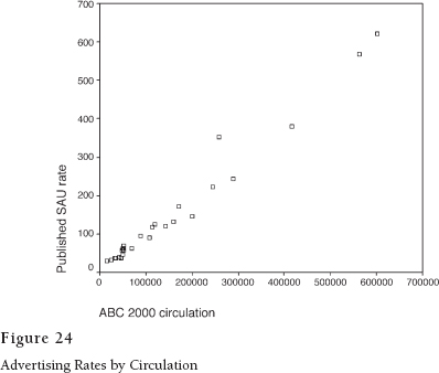
The basic requirement is to have two variables that can be measured on some continuum. Not every interesting thing can be measured in that way, but many things important to business people—dollars and cents, for example—do meet the requirement. Here is one example: newspaper advertising rates and circulation.

Are they related? Common sense tells us that they should be, and we can check by drawing a plot that shows the position of different newspapers on the two dimensions. In Figure 24, circulation is measured along the horizontal axis and advertising rate (expressed in Standard Advertising Units) along the vertical. They form a pattern that looks a lot like a straight line.

Using a method developed by Karl Pearson (1857–1936), we can find the line that best describes that pattern. It is called the least squares line because it minimizes the vertical squared difference between each newspaper and the line. Figure 25 shows the plot again with the line drawn in. This line helps us in a couple of ways. Its slope tells us how much advertising rates increase for each unit of circulation. The value of the slope is .001, meaning that published ad rates tend to go up by one-tenth of a cent for each unit of circulation.

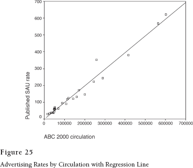
The amount of scatter around the line provides a cue to how much error we would make if we follow the tenth-of-a-cent rule to predict the ad prices of individual newspapers for which we already knew the circulation. If there is no scatter around the line, i.e. all the newspapers are spot on, then prediction would be perfect and Pearson's correlation coefficient would be one.

For this particular case of newspaper circulation and ad rates, it is almost one. To be exact, it is .985.

When we square the correlation coefficient, we have a measure of the variation in SAU rates that is predicted or “explained” by circulation. The square of .985 is .97. In other words, having the information about circulation enables us to guess the ad rates of papers in the sample with ninety-seven percent greater accuracy than we would obtain by using the mean for our estimate.

Predicting ad rates from circulation is no great achievement, but the variation that is left over might be interesting. Pearson's method lets us see it in picture form. Look at the data point that is farthest above the line (at about 258,000 circulation and between $300 and $400 on the SAU scale). According to the regression formula, that paper's managers ought to be asking about $250 per SAU. Instead, they get away with around $100 more. If we could find out how they do that, we might have some useful information for the newspaper industry.

The difference between the expected value (based on the regression line) and the observed value is called the “residual.” Think of it as left-over variation after the explanatory power of circulation size has been all used up. We can use that information by taking the residuals for all the papers in the plot and use them as the variable to explore in a new plot with a new explanatory variable. Pearson figured out how to do this with many different explanatory (or “independent”) variables in a procedure that was difficult in his day but is easy with a computer. It is called multiple regression, and it estimates the effects of different explanatory variables after the effects of the others have been taken into account.

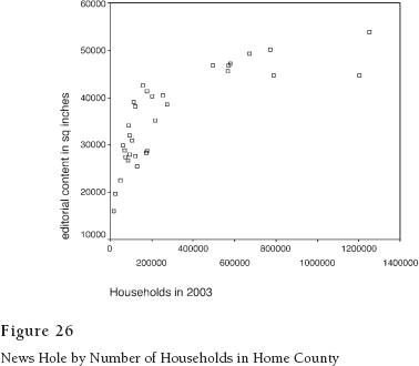
As you perhaps have noticed at this stage in your life, God did not make the world in straight lines. Consider, for example, the effect of market size on volume of news-editorial content (Figure 26).

The amount of news increases steeply with market size until size exceeds 400,000 households. After that, it levels off. If we want to use the linear model, we have two choices. We can treat the markets with less than 400,000 as a separate population and set the others aside. Or, we can re-express market size as its logarithm. The advantage of the latter strategy is that we can still use straight-line statistics, but with recognition that what we are really dealing with is a curve—and a very specific curve at that.

Figure 27 shows the same plot with the re-expression; it is much closer to a straight line. Before computers made this so easy, we made plots like this by hand on log graph paper. On the base-ten log scale, the values from one to ten occupy the same linear space as those from ten to one hundred or those from one hundred to one thousand. In other words, the scale is stretched out on the low end and compressed at the high end. It's as though the previous graph were printed on a rubber sheet, and we stretched the left and compressed the right to straighten the line.

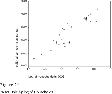
Isn't this cheating? No. It would be cheating to pretend that the original line was straight. Now we have a cleaner mathematical description of the world as it really is. And the correlation coefficient is .907, which is about as good as it gets. The log of households explains eighty-two percent of the variance in news hole.

When we use regression methods, we are trying to explain variance around the mean of the dependent variable. We do it by looking for covariance—the degree to which two measured things vary together. If we know a lot about these variables and the situations in which we find them, we might even start to make some assumptions about causation. But correlation is not by itself enough to prove cause and effect. No statistical procedure can do that. In the end, we are left with judgment based on our observations, knowledge, and experience with the real world. We still have stuff to argue about. But with the discipline of statistics, as Robert P. Abelson has said, it is “principled argument.”

Because most of the data examined in this book use continuous rather than categorical measurement, my arguments are based mostly on correlations. Usually, I report the variance explained (r²) in the text, because it is a more intuitive figure, and put the correlation coefficient (r) in the footnote. Also left to the footnote in most cases is the statistical significance of the correlation, expressed as the probability that the relationship is due to chance.

Sometimes when trying to determine the direction of causation, I use partial correlations. A partial correlation estimates the relationship between two variables after the effect of a third variable that influences them both has been accounted for. This procedure sometimes helps because it can rule out the possibility that some third variable is causing the relationship between the two under investigation. For example, market size is a fertile variable that can make the many things that it causes seem to be related on their own when they are really independent.

When dealing with correlation, it's always a good idea to look at the scatter-plot to see if the result is being driven by one or two eccentric cases or if the relationship is nonlinear. This is especially true for small samples like those used in this book. I have included many scatterplots for that reason, as well as to give the reader an intuitive appreciation of the argument that community influence and newspaper success are related.