2.1 Time Series Data
A time series orders observations
Time series can be measured at different frequencies
Time series exhibit different patterns of ‘persistence’
Historical time can matter
A short annual time series
Date | 2012 | 2013 | 2014 | 2015 | 2016 | 2017 |
Value | 4 | 6 | 5 | 9 | 7 | 3 |
The most important property of a time series is the ordering of observations by ‘time’s arrow’: the value in 2014 happened before that in 2015. We live in a world where we seem unable to go back into the past, to undo a car crash, or a bad investment decision, notwithstanding science-fiction stories of ‘time-travellers’. That attribute will be crucial, as time-series analysis seeks to explain the present by the past, and forecast the future from the present. That last activity is needed as it also seems impossible to go into the future and return with knowledge of what happens there.
Time Series Occur at Different Frequencies
A second important feature is the frequency at which a time series is recorded, from nano-seconds in laser experiments, every second for electricity usage, through days for rainfall, weeks, months, quarters, years, decades and centuries to millenia in paleo-climate measures. It is relatively easy to combine higher frequencies to lower, as in adding up the economic output of a country every quarter to produce an annual time series. An issue of concern to time-series analysts is whether important information is lost by such temporal aggregation. Using a somewhat stretched example, a quarterly time series that went 2, 5, 9, 4 then 3, 4, 8, 5 and so on, reveals marked changes with a pattern where the second ‘half’ is much larger than the ‘first’, whereas the annual series is always just a rather uninformative 20. The converse of creating a higher-frequency series from a lower is obviously more problematic unless there are one or more closely related variables measured at the higher frequency to draw on. For example, monthly measures of retail sales may help in creating a monthly series of total consumers’ expenditure from its quarterly time series. In July 2018, the United Kingdom Office for National Statistics started producing monthly aggregate time series, using electronic information that has recently become available to it.
Time Series Exhibit Patterns of ‘Persistence’

Panel (a) UK annual unemployment rate, 1860–2017; (b) a sequence of random numbers
Figure 2.1 illustrates two very different time series. The top panel records the annual unemployment rate in the United Kingdom from 1860–2017. The vertical axis records the rate (e.g., 0.15 is 15%), and the horizontal axis reports the time. As can be seen (we call this ocular econometrics), when unemployment is high, say above the long-run mean of 5% as from 1922–1939, it is more likely to be high in the next year, and similarly when it is low, as from 1945–1975, it tends to stay low. By way of contrast, the lower panel plots some computer generated random numbers between  and
and  , where no persistence can be seen.
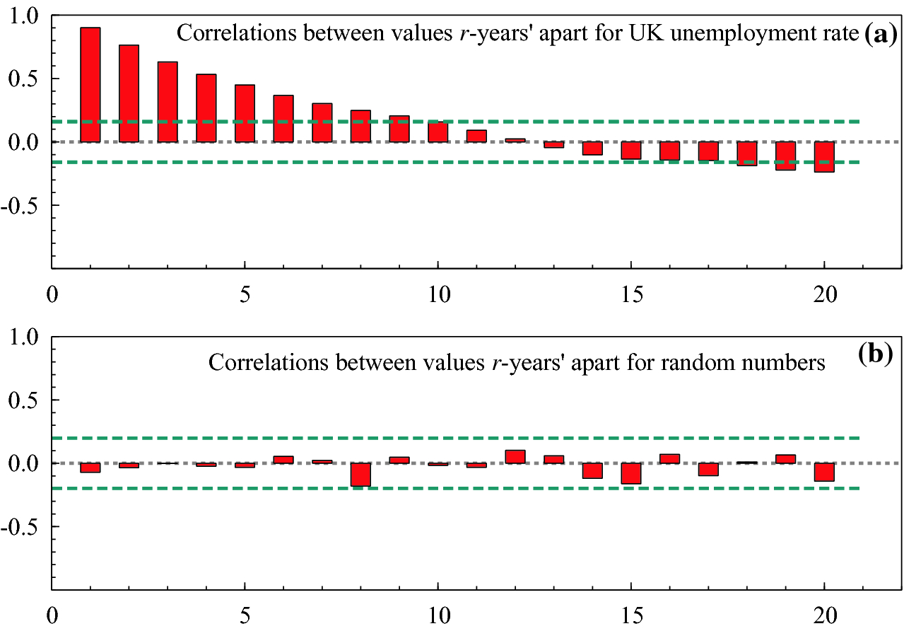
Correlations between successively futher apart observations: (a) UK unemployment rates; (b) random numbers
Historical Time can Matter
Historical time is often an important attribute of a time series, so it matters that an event occurred in 1939 (say) rather than 1956. This leads to our second primer concerned with a very fundamental property of all time series: does it ‘look essentially the same at different times’, or does it evolve? Examples of relatively progressive evolution include technology, medicine, and longevity, where the average age of death in the western world has increased at about a weekend every week since around 1860. But major abrupt and often unexpected shifts can also occur, as with financial crises, earthquakes, volcanic eruptions or a sudden slow down in improving longevity as seen recently in the USA.
2.2 Stationarity and Non-stationarity
A time series is not stationary if historical time matters
Sources of non-stationarity
Historical review of understanding non-stationarity
We all know what it is like to be stationary when we would rather be moving: sometimes stuck in traffic jams, or still waiting at an airport long after the scheduled departure time of our flight. A feature of such unfortunate situations is that the setting ‘looks the same at different times’: we see the same trees beside our car until we start to move again, or the same chairs in the airport lounge. The word stationary is also used in a more technical sense in statistical analyses of time series: a stationary process is one where its mean and variance stay the same over time. Our solar system appears to be almost stationary, looking essentially the same over our lives (though perhaps not over very long time spans).
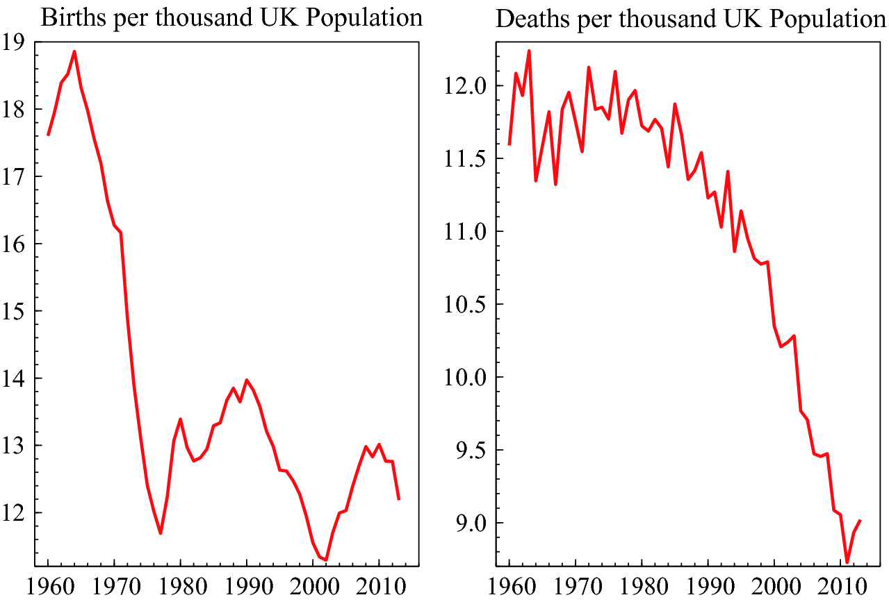
Births and deaths per thousand of the UK population
As a corollary, a non-stationary process is one where the distribution of a variable does not stay the same at different points in time–the mean and/or variance changes–which can happen for many reasons. Stationarity is the exception and non-stationarity is the norm for most social science and environmental times series. Specific events can matter greatly, including major wars, pandemics, and massive volcanic eruptions; financial innovation; key discoveries like vaccination, antibiotics and birth control; inventions like the steam engine, dynamo and flight; etc. These can cause persistent shifts in the means and variances of the data, thereby violating stationarity. Figure 2.3 shows the large drop in UK birth rates following the introduction of oral contraception, and the large declines in death rates since 1960 due to increasing longevity. Comparing the two panels shows that births exceeded deaths at every date, so the UK population must have grown even before net immigration is taken into account.
Economies evolve and change over time in both real and nominal terms, sometimes dramatically as in major wars, the US Great Depression after 1929, the ‘Oil Crises’ of the mid 1970s, or the more recent ‘Financial Crisis and Great Recession’ over 2008–2012.
Sources of Non-stationarity
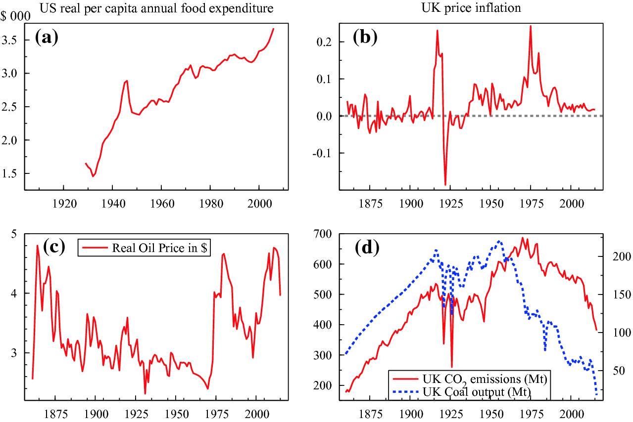
(a) US real per capita annual food expenditure in $000; (b) UK price inflation; (c) Real oil price in $ (log scale); (d) UK coal output (right-hand axis) and CO emissions (left-hand axis), both in millions of tons (Mt) per annum
 emissions (solid line), both in Mt per annum: what goes up can come down. The fall in the former from 250 Mt per annum to near zero is as dramatic a non-stationarity as one could imagine, as is the behaviour of emissions, with huge ‘outliers’ in the 1920s and a similar ‘
 ’ shape. In per capita terms, the UK’s CO
 emissions are now below any level since 1860–when the UK was the workshop of the world.
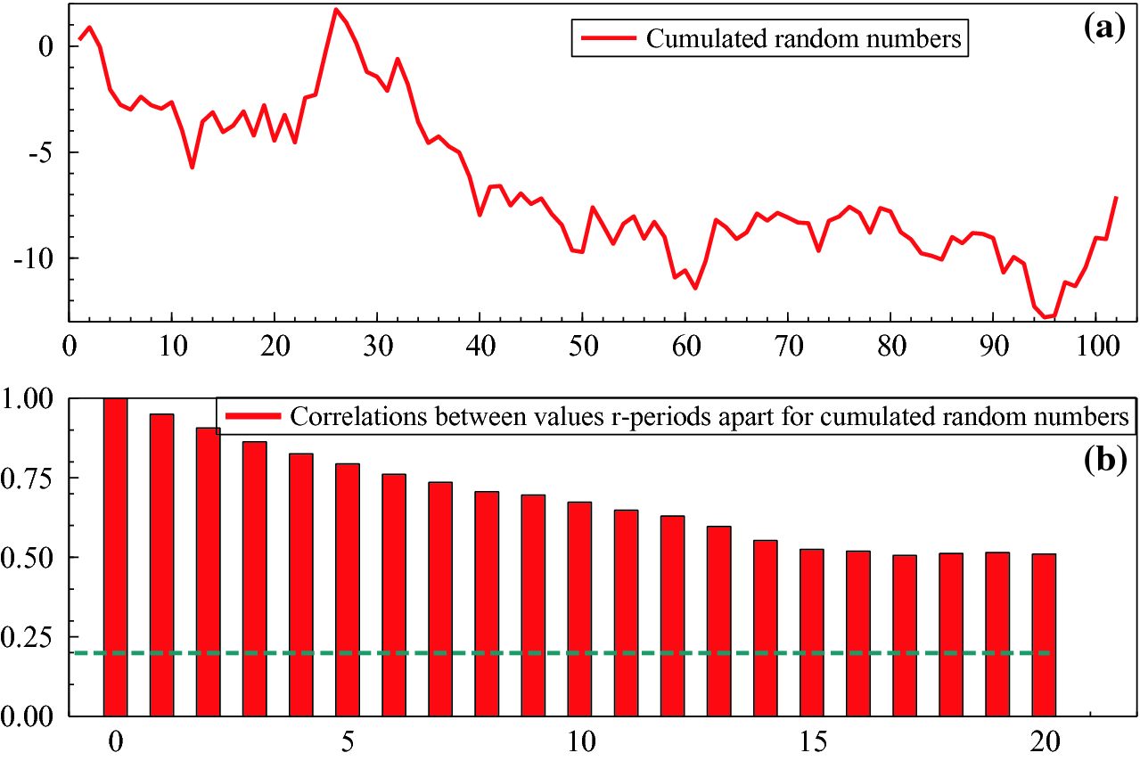
(a) Time series of the cumulated random numbers; (b) correlations between successively futher apart observations
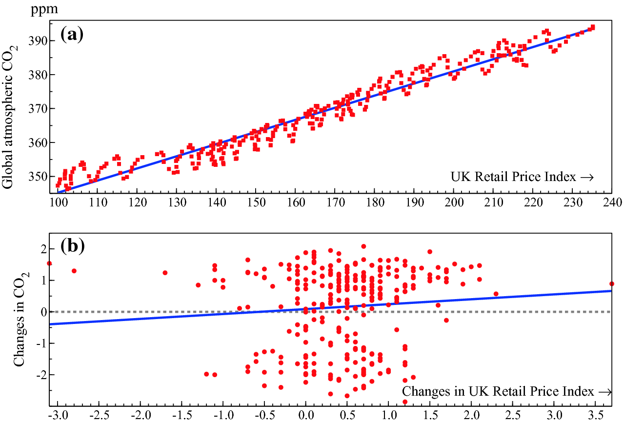
(a) ‘Explaining’ global levels of atmospheric CO by the UK retail price index (RPI); (b) no relation between their changes
Empirical modelling relating variables faces important difficulties when time series are non-stationary. If two unrelated time series are non-stationary because they evolve by accumulating past shocks, their correlation will nevertheless appear to be significant about 70% of the time using a conventional 5% decision rule.
Apocryphal examples during the Victorian era were the surprising high positive correlations between the numbers of human births and storks nesting in Stockholm, and between murders and membership of the Church of England. As a consequence, these are called nonsense relations. A silly example is shown in Fig. 2.6(a) where the global atmospheric concentrations of CO are ‘explained’ by the monthly UK Retail Price Index (RPI), partly because both have increased over the sample, 1988(3) to 2011(6). However, Panel (b) shows that the changes in the two series are essentially unrelated.
The nonsense relations problem arises because uncertainty is seriously under-estimated if stationarity is wrongly assumed. During the 1980s, econometricians established solutions to this problem, and en-route also showed that the structure of economic behaviour virtually ensured that most economic data would be non-stationary. At first sight, this poses many difficulties for modelling economic data. But we can use it to our advantage as such non-stationarity is often accompanied by common trends. Most people make many more decisions (such as buying numerous items of shopping), than the small number of variables that guide their decisions (e.g., their income or bank balance). That non-stationary data often move closely together due to common variables driving economic decisions enables us to model the non-stationarities. Below, we will use the behaviour of UK wages, prices, productivity and unemployment over 1860–2016 to illustrate the discussion and explain empirical modelling methods that handle non-stationarities which arise from cumulating shocks.
Many economic models used in empirical research, forecasting or for guiding policy have been predicated on treating observed data as stationary. But policy decisions, empirical research and forecasting also must take the non-stationarity of the data into account if they are to deliver useful outcomes. We will offer guidance for policy makers and researchers on identifying what forms of non-stationarity are prevalent, what hazards each form implies for empirical modelling and forecasting, and for any resulting policy decisions, and what tools are available to overcome such hazards.
Historical Review of Understanding Non-stationarity
Developing a viable analysis of non-stationarity in economics really commenced with the discovery of the problem of ‘nonsense correlations’.These high correlations are found between variables that should be unrelated: for example, that between the price level in the UK and cumulative annual rainfall shown in Hendry (1980).3 Yule (1897) had considered the possibility that both variables in a correlation calculation might be related to a third variable (e.g., population growth), inducing a spuriously high correlation: this partly explains the close relation in Fig. 2.6. But by Yule (1926), he recognised the problem was indeed ‘nonsense correlations’. He suspected that high correlations between successive values of variables, called serial, or auto, correlation as in Fig. 2.5(b), might affect the correlations between variables. He investigated that in a manual simulation experiment, randomly drawing from a hat pieces of paper with digits written on them. He calculated correlations between pairs of draws for many samples of those numbers and also between pairs after the numbers for each variable were cumulated once, and finally cumulated twice. For example, if the digits for the first variable went 5, 9, 1, 4,  , the cumulative numbers would be 5, 14, 15, 19,
  and so on. Yule found that in the purely random case, the correlation coefficient was almost normally distributed around zero, but after the digits were cumulated once, he was surprised to find the correlation coefficient was nearly uniformly distributed, so almost all correlation values were equally likely despite there being no genuine relation between the variables. Thus, he found ‘significant’, though not very high, correlations far more often than for non-cumulated samples. Yule was even more startled to discover that the correlation coefficient had a U-shaped distribution when the numbers were doubly cumulated, so the correct hypothesis of no relation between the genuinely unrelated variables was virtually always rejected due to a near-perfect, yet nonsense, correlation of
  .
.
Granger and Newbold (1974) re-emphasized that an apparently ‘significant relation’ between variables, but where there remained substantial serial correlation in the residuals from that relation, was a symptom associated with nonsense regressions. Phillips (1986) provided a technical analysis of the sources and symptoms of nonsense regressions. Today, Yule’s three types of time series are called integrated of order zero, one, and two respectively, usually denoted I(0), I(1), and I(2), as the number of times the series integrate (i.e., cumulate) past values. Conversely, differencing successive values of an I(1) series delivers an I(0) time series, etc., but loses any information connecting the levels. At the same time as Yule, Smith (1926) had already suggested that a solution was nesting models in levels and differences, but this great step forward was quickly forgotten (see Terence Mills 2011). Indeed, differencing is not the only way to reduce the order of integration of a group of related time series, as Granger (1981) demonstrated with the introduction of the concept of cointegration, extended by Engle and Granger (1987) and discussed in Sect. 4.2: see Hendry (2004) for a history of the development of cointegration.
The history of structural breaks–the topic of the next ‘primer’–has been less studied, but major changes in variables and consequential shifts between relationships date back to at least the forecast failures that wrecked the embryonic US forecasting industry (see Friedman 2014). In considering forecasting the outcome for 1929–what a choice of year!–Smith (1929) foresaw the major difficulty as being unanticipated location shifts (although he used different terminology), but like his other important contribution just noted, this insight also got forgotten. Forecast failure has remained a recurrent theme in economics with notable disasters around the time of the oil crises (see e.g., Perron 1989) and the ‘Great Recession’ considered in Sect. 7.3.
What seems to have taken far longer to realize is that to every forecast failure there is an associated theory failure as emphasized by Hendry and Mizon (2014), an important issue we will return to in Sect. 4.4.4 Meantime, we consider the other main form of non-stationarity, namely the many forms of ‘structural breaks’.
2.3 Structural Breaks
Types of structural breaks
Causes of structural breaks
Consequences of structural breaks
Tests for structural breaks
Modelling facing structural breaks
Forecasting in processes with structural breaks
Regime-shift models
A structural break denotes a shift in the behaviour of a variable over time, such as a jump in the money stock, or a change in a previous relationship between observable variables, such as between inflation and unemployment, or the balance of trade and the exchange rate. Many sudden changes, particularly when unanticipated, cause links between variables to shift. This is a problem that is especially prevalent in economics as many structural breaks are induced by events outside the purview of most economic analyses, but examples abound in the sciences and social sciences, e.g., volcanic eruptions, earthquakes, and the discovery of penicillin. The consequences of not taking breaks into account include poor models, large forecast errors after the break, mis-guided policy, and inappropriate tests of theories.
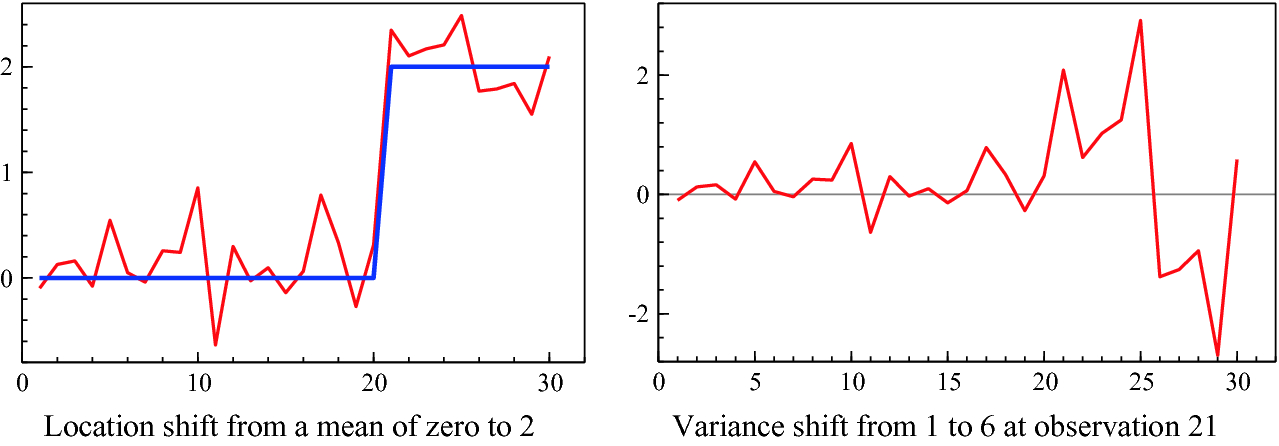
Such breaks can take many forms. The simplest to visualize is a shift in the mean of a variable as shown in the left-hand panel of Fig. 2.7. This is a ‘location shift’, from a mean of zero to 2. Forecasts based on the zero mean will be systematically badly wrong.
Next, a shift in the variance of a time series is shown in the right-hand graph of Fig. 2.7. The series is fairly ‘flat’ till about observation 19, then varies considerably more after.
Two examples of structural breaks
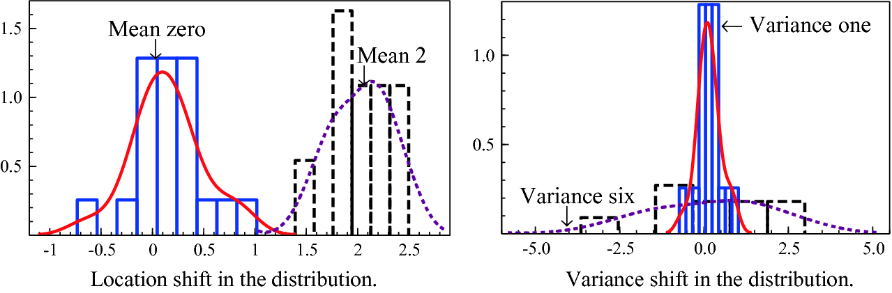
The impacts on the statistical distributions of the two examples of structural breaks
Distributional shifts certainly occur in the real world, as Fig. 2.9 shows, plotting four sub-periods of annual UK CO emissions in Mt. The first three sub-periods all show the centers of the distributions moving to higher values, but the fourth (1980–2016) jumps back below the previous sub-period distribution.
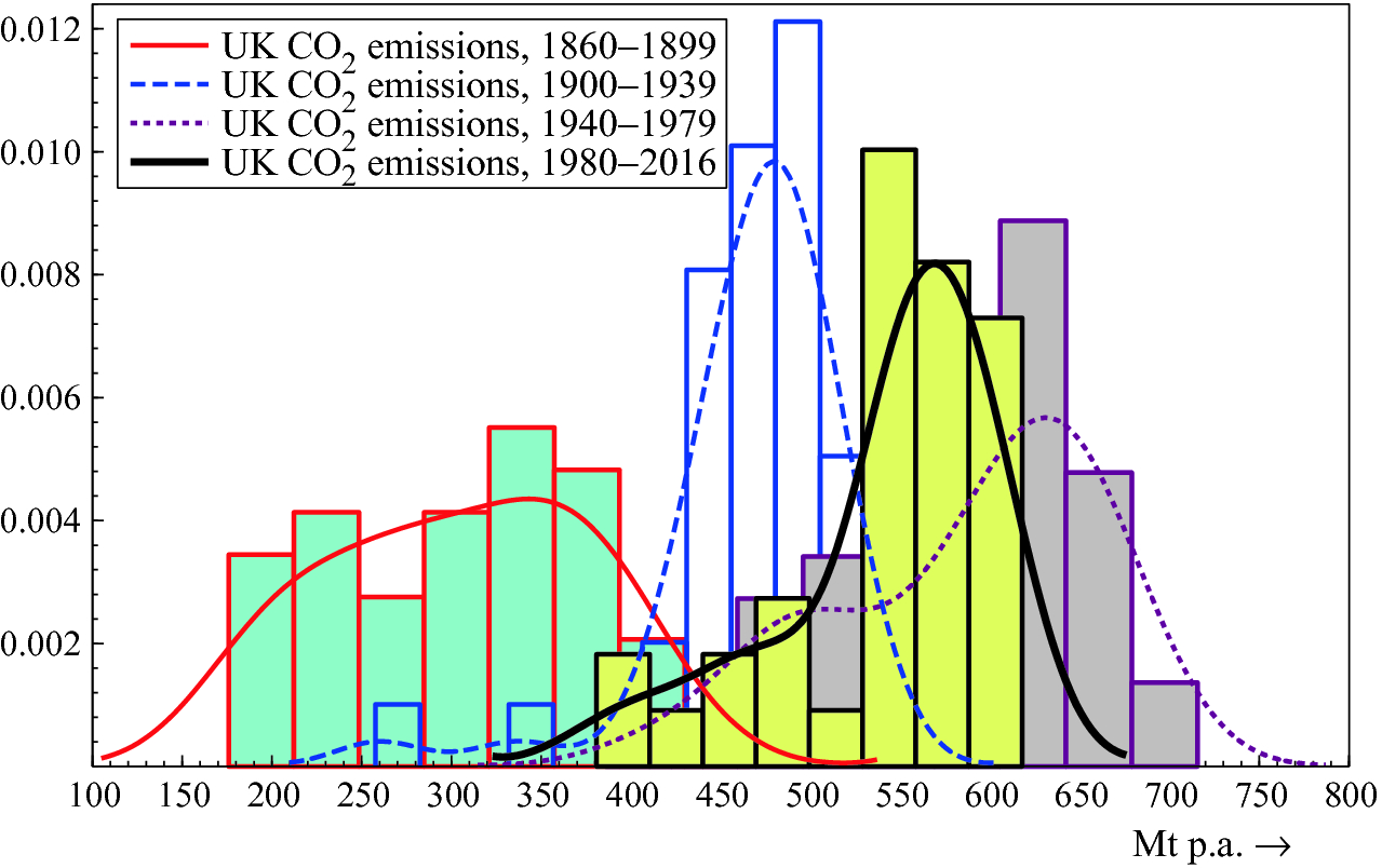
Distributional shifts of total UK CO emissions, Mt p.a.
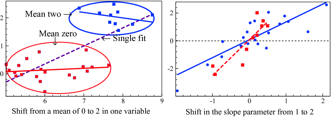
The impacts on statistical relationships of shifts in mean and slope parameters
Causes of Structural Breaks
The world has changed enormously in almost every measurable way over the last few centuries, sometimes abruptly (for a large body of evidence, see the many time series in https://ourworldindata.org/). Of the numerous possible instances, dramatic shifts include World War I; the 1918–20 flu’ epidemic; 1929 crash and ensuing Great Depression; World War II; the 1970s oil crises; 1997 Asian financial crisis; the 2000 ‘dot com’ crash; and the 2008–2012 financial crisis and Great Recession (and maybe Brexit). Such large and sudden breaks usually lead to location shifts. More gradual changes can cause the parameters of relationships to ‘drift’: changes in technology, social mores, or legislation usually take time to work through.
Consequences of Structural Breaks
The impacts of structural breaks on empirical models naturally depend on their forms, magnitudes, and numbers, as well as on how well specified the model in question is. When large location shifts or major changes in the parameters linking variables in a relationship are not handled correctly, statistical estimates of relations will be distorted. As we discuss in Chapter 7, this often leads to forecast failure, and if the ‘broken’ relation is used for policy, the outcomes of policy interventions will not be as expected. Thus, viable relationships need to account for all the structural breaks that occurred, even though in practice, there will be an unknown number, most of which will have an unknown magnitude, form, and duration and may even have unknown starting and ending dates.
Tests for Structural Breaks
There are many tests for structural breaks in given relationships, but these often depend not only on knowing the correct relationship to be tested, but also on knowing a considerable amount about the types of breaks, and the properties of the time series being analyzed. Tests include those proposed by Brown et al. (1975), Chow (1960), Nyblom (1989), Hansen (1992a), Hansen (1992b) (for I(1) data), Jansen and Teräsvirta (1996), and Bai and Perron (1998, 2003). Perron (2006) provided a wide ranging survey of then available methods of estimation and testing in models with structural breaks, including their close links to processes with unit roots, which are non-stationary stochastic processes (discussed above) that can cause problems in statistical inference. To apply any test requires that the model is already specified, so while it is certainly wise to test if there are important structural breaks leading to parameter non-constancies, their discovery then reveals the model to be flawed, and how to ‘repair’ it is always unclear. Tests can reject because of other untreated problems than the one for which they were designed: for example, apparent non-constancy may be due to residual autocorrelation, or unmodelled persistence left in the unexplained component, which distorts the estimated standard errors (see e.g., Corsi et al. 1982). A break can occur because an omitted determinant shifts, or from a location shift in an irrelevant variable included inadvertently, and the ‘remedy’ naturally differs between such settings.
Modelling Facing Structural Breaks
Failing to model breaks will almost always lead to a badly-specified empirical model that will not usefully represent the data. Knowing of or having detected breaks, a common approach is to ‘model’ them by adding appropriate indicator variables, namely artificial variables that are zero for most of a sample period but unity over the time that needs to be indicated as having a shift: Fig. 2.7 illustrates a step indicator that takes the value 2 for observations 21–30. Indicators can be formulated to reflect any relevant aspect of a model, such as changing trends, or multiplied by variables to capture when parameters shift, and so on. It is possible to design model selection strategies that tackle structural breaks automatically as part of their algorithm, as advocated by Hendry and Doornik (2014). Even though such approaches, called indicator saturation methods (see Johansen and Nielsen 2009; Castle et al. 2015), lead to more candidate explanatory variables than there are available observations, it is possible for a model selection algorithm to include large blocks of indicators for any number of outliers and location shifts, and even parameter changes (see e.g., Ericsson 2012). Indicators relevant to the problem at hand can be designed in advance, as with the approach used to detect the impacts of volcanic eruptions on temperature in Pretis et al. (2016).
Forecasting in Processes with Structural Breaks
In the forecasting context, not all structural breaks matter equally, and indeed some have essentially no effect on forecast accuracy, but may change the precision of forecasts, or estimates of forecast-error variances. Clements and Hendry (1998) provide a taxonomy of sources of forecast errors which explains why location shifts—changes in the previous means, or levels, of variables in relationships—are the main cause of forecast failures. Ericsson (1992) provides a clear discussion. Figure 2.7 again illustrates why the previous mean provides a very poor forecast of the final 10 data points. Rapid detection of such shifts, or better still, forecasting them in advance, can reduce systematic forecast failure, as can a number of devices for robustifying forecasts after location shifts, such as intercept corrections and additional differencing, the topic of Chapter 7.
Regime-Shift Models
An alternative approach models shifts, including recessions, as the outcome of stochastic shocks in non-linear dynamic processes, the large literature on which was partly surveyed by Hamilton (2016). Such models assume there is a probability at any point in time, conditional on the current regime and possibly several recent past regimes, that an economy might switch to a different state. A range of models have been proposed that could characterize such processes, which Hamilton describes as ‘a rich set of tools and specifications on which to draw for interpreting data and building economic models for environments in which there may be changes in regime’. However, an important concern is which specification and which tools apply in any given instance, and how to choose between them when a given model formulation is not guaranteed to be fully appropriate. Consequently, important selection and evaluation issues must be addressed.
2.4 Model Selection
What is model selection?
Evaluating empirical models
Objectives of model selection
Model selection methods
Concepts used in analyses of statistical model selection
Consequences of statistical model selection
Model selection concerns choosing a formal representation of a set of data from a range of possible specifications thereof. It is ubiquitous in observational-data studies because the processes generating the data are almost never known. How selection is undertaken is sometimes not described, and may even give the impression that the final model reported was the first to be fitted. When the number of candidate variables needing analyzed is larger than the available sample, selection is inevitable as the complete model cannot be estimated. In general, the choice of selection method depends on the nature of the problem being addressed and the purpose for which a model is being sought, and can be seen as an aspect of testing multiple hypotheses: see Lehmann (1959). Purposes include understanding links between data series (especially how they evolved over the past), to test a theory, to forecast future outcomes, and (in e.g., economics and climatology) to conduct policy analyses.
It might be thought that a single ‘best’ model (on some criteria) should resolve all four purposes, but that transpires not to be the case, especially when observational data are not stationary. Indeed, the set of models from which one is to be selected may be implicit, as when the functional form of the relation under study is not known (linear, log-linear or non-linear), or when there may be an unknown number of outliers, or even shifts. Model selection can also apply to the design of experiments such that the data collected is well-suited to the problem. As Konishi and Kitagawa (2008, p. 75) state, ‘The majority of the problems in statistical inference can be considered to be problems related to statistical modeling’. Relatedly, Sir David Cox (2006, p. 197) has said, ‘How [the] translation from subject-matter problem to statistical model is done is often the most critical part of an analysis’.
Evaluating Empirical Models
Irrespective of how models are selected, it is always feasible to evaluate any chosen model against the available empirical evidence. There are two main criteria for doing so in our approach, congruence and encompassing .
The first concerns how well the model fits the data, the theory and any constraints imposed by the nature of the observations. Fitting the data requires that the unexplained components, or residuals, match the properties assumed for the errors in the model formulation. These usually entail no systematic behaviour, such as successive residuals being correlated (serial or autocorrelation), that the residuals are relatively homogeneous in their variability (called homoscedastic), and that all parameters which are assumed to be constant over time actually are. Matching the theory requires that the model formulation is consistent with the analysis from which it is derived, but does not require that the theory model is imposed on the data, both because abstract theory may not reflect the underlying behaviour, and because little would be learned if empirical results merely put ragged cloth on a sketchy theory skeleton. Matching intrinsic data properties may involve taking logarithms to ensure an inherently positive variable is modelled as such, or that flows cumulate correctly to stocks, and that outcomes satisfy accounting constraints.
Although satisfying all of these requirements may seem demanding, there are settings in which they are all trivially satisfied. For example, if the data are all orthogonal, and independent identically distributed (IID)—such as independent draws from a Normal distribution with a constant mean and variance and no data constraints—all models would appear to be congruent with whatever theory was used in their formulation. Thus, an additional criterion is whether a model can encompass, or explain the results of, rival explanations of the same variables. There is a large literature on alternative approaches, but the simplest is parsimonious encompassing in which an empirical model is embedded within the most general formulation (often the union of all the contending models) and loses no significant information relative to that general model. In the orthogonal IID setting just noted, a congruent model may be found wanting because some variables it excluded are highly significant statistically when included. That example also emphasizes that congruence is not definitive, and most certainly is not ‘truth’, in that a sequence of successively encompassing congruent empirical models can be developed in a progressive research strategy: see Mizon (1984, 2008), Hendry (1988, 1995), Govaerts et al. (1994), Hoover and Perez (1999), Bontemps and Mizon (2003, 2008), and Doornik (2008).
Objectives of Model Selection
At base, selection is an attempt to find all the relevant determinants of a phenomenon usually represented by measurements on a variable, or set of variables, of interest, while eliminating all the influences that are irrelevant for the problem at hand. This is most easily understood for relationships between variables where some are to be ‘explained’ as functions of others, but it is not known which of the potential ‘explaining’ variables really matter. A simple strategy to ensure all relevant variables are retained is to always keep every candidate variable; whereas to ensure no irrelevant variables are retained, keep no variables at all. Manifestly these strategies conflict, but highlight the ‘trade-off’ that affects all selection approaches: the more likely a method is to retain relevant influences by some criterion (such as statistical significance) the more likely some irrelevant influences will chance to be retained. The costs and benefits of that trade-off depend on the context, the approach adopted, the sample size, the numbers of irrelevant and relevant variables—which are unknown—how substantive the latter are, as well as on the purpose of the analysis.
For reliably testing a theory, the model must certainly include all the theory-relevant variables, but also all the variables that in fact affect the outcomes being modelled, whereas little damage may be done by also including some variables that are not actually relevant. However, for forecasting, even estimating the in-sample process that generated the data need not produce the forecasts with the smallest mean-square errors (see e.g., Clements and Hendry 1998). Finally, for policy interventions, it is essential that the relation between target and instrument is causal, and that the parameters of the model in use are also invariant to the intervention if the policy change is to have the anticipated effect. Here the key concept is of invariance under changes, so shifts in the policy variable, say a price rise intended to increase revenue from sales, does not alter consumers’ attitudes to the company in question, thereby shifting their demand functions and so leading to the unintended consequence of a more than proportionate fall in sales.
Model Selection Methods
Most empirical models are selected by some process, varying from imposing a theory-model on the data evidence (having ‘selected’ the theory), through manual choice, which may be to suit an investigator’s preferences, to when a computer algorithm such as machine learning is used. Even in this last case, there is a large range of possible approaches, as well as many choices as to how each algorithm functions, and the different settings in which each algorithm is likely to work well or badly—as many are likely to do for non-stationary data. The earliest selection approaches were manual as no other methods were on offer, but most of the decisions made during selection were then undocumented (see the critique in Leamer 1978), making replication difficult. In economics, early selection criteria were based on the ‘goodness-of-fit’ of models, pejoratively called ‘data mining’, but Gilbert (1986) highlighted that a greater danger of selection was its being used to suppress conflicting evidence. Statistical analyses of selection methods have provided many insights: e.g., Anderson (1962) established the dominance of testing from the most general specification and eliminating irrelevant variables relative to starting from the simplest and retaining significant ones. The long list of possible methods includes, but is not restricted to, the following, most of which use parsimony (in the sense of penalizing larger models) as part of their choice criteria.
Information criteria have a long history as a method of choosing between alternative models. Various information criteria have been proposed, all of which aim to choose between competing models by selecting the model with the smallest information loss. The trade-off between information loss and model ‘complexity’ is captured by the penalty, which differs between information criteria. For example, the AIC proposed by Akaike (1973), sought to balance the costs when forecasting from a stationary infinite autoregression of estimation variance from retaining small effects against the squared bias of omitting them. Schwarz (1978) SIC (also called BIC, for Bayesian information criterion), aimed to consistently estimate the parameters of a fixed, finite-dimensional model as the sample size increased to infinity. HQ, from Hannan and Quinn (1979), established the smallest penalty function that will deliver the same outcome as SIC in very large samples. Other variants of information criteria include focused criteria (see Claeskens and Hjort 2003), and the posterior information criterion in Phillips and Ploberger (1996).
Variants of selection by goodness of fit include choosing by the maximum multiple correlation coefficient (criticised by Lovell 1983); Mallows (1973)  criterion; step-wise regression (see e.g., Derksen and Keselman 1992, which Leamer called ‘unwise’), which is a class of single-path search procedures for (usually) adding variables one at a time to a regression (e.g., including the next variable with the highest remaining correlation), only retaining significant estimated parameters, or dropping the least significant remaining variables in turn.
Penalised-fit approaches like shrinkage estimators, as in James and Stein (1961), and the Lasso (least absolute shrinkage and selection operator) proposed by Tibshirani (1996) and Efron et al. (2004). These are like step-wise with an additional penalty for each extra parameter.
Bayesian selection methods which often lead to model averaging: see Raftery (1995), Phillips (1995), Buckland et al. (1997), Burnham and Anderson (2002), and Hoeting et al. (1999), and Bayesian structural time series (BSTS: Scott and Varian 2014).
Automated general-to-specific (Gets) approaches as in Hoover and Perez (1999), Hendry and Krolzig (2001), Doornik (2009), and Hendry and Doornik (2014). This approach will be the one mainly used in this book when we need to explicitly select a model from a larger set of candidates, especially when there are more such candidates than the number of observations.
Model selection also has many different designations, such as subset selection (Miller 2002), and may include computer learning algorithms.
Concepts for analyses of statistical model selection
There are also many different concepts employed in the analyses of statistical methods of model selection. Retention of irrelevant variables is often measured by the ‘false-positives rate’ or ‘false-discovery rate’ namely, how often irrelevant variables are incorrectly selected by a test adventitiously rejecting the null hypothesis of irrelevance. If a test is correctly calibrated (which unfortunately is often not the case for many methods of model selection, such as step-wise), and has a nominal significance level of (say) 1%, it should reject the null hypothesis incorrectly 1% of the time (Type-I error). Thus, if 100 such tests are conducted under the null, 1 should reject by chance on average (i.e.,  ). Hendry and Doornik (2014) refer to the actual retention rate of irrelevant variables during selection as the empirical gauge and seek to calibrate their algorithm such that the gauge is close to the nominal significance level. Johansen and Nielsen (2016) investigate the distribution of estimates of the gauge. Bayesian approaches often focus on the concept of ‘model uncertainty’, essentially the probability of selecting closely similar models that nevertheless lead to different conclusions. With 100 candidate variables, there are
  possible models generated by every combination of the 100 variables, creating great scope for such model uncertainty. Nevertheless, when all variables are irrelevant, on average 1 variable would be retained at 1%, so model uncertainty has been hugely reduced from a gigantic set of possibilities to a tiny number. Although different irrelevant variables will be selected adventitiously in different draws, this is hardly a useful concept of ‘model uncertainty’.
The more pertinent difficulty is finding and retaining relevant variables, which depends on how substantive their influence is. If a variable would not be retained by the criterion in use even when it was the known sole relevant variable, it will usually not be retained by selection from a larger set. Crucially, a relevant variable can only be retained if it is in the candidate set being considered, so indicators for outliers and shifts will never be found unless they are considered. One strategy is to always retain the set of variables entailed by the theory that motivated the analysis while selecting from other potential determinants, shift effects etc., allowing model discovery jointly with evaluating the theory (see Hendry and Doornik 2014).
Consequences of Statistical Model Selection
Selection of course affects the statistical properties of the resulting estimated model, usually because only effects that are ‘significant’ at the pre-specified level are retained. Thus, which variables are selected varies in different samples and on average, estimated coefficients of retained relevant variables are biased away from the origin. Retained irrelevant variables are those that chanced to have estimated coefficients far from zero in the particular data sample. The former are often called ‘pre-test biases’ as in Judge and Bock (1978). The top panel in Fig. 2.11 illustrates when  denotes the distribution without selection, and
  with selection requiring significance at 5%. The latter distribution is shifted to the right and has a mean
 ![$$\mathsf{E}[\widetilde{b}]$$](../images/479794_1_En_2_Chapter/479794_1_En_2_Chapter_TeX_IEq30.png) of 0.276 when the unselected mean
of 0.276 when the unselected mean ![$$\mathsf{E}[\widehat{b}]$$](../images/479794_1_En_2_Chapter/479794_1_En_2_Chapter_TeX_IEq31.png) is 0.2, leading to an upward bias of 38%.
is 0.2, leading to an upward bias of 38%.
 to
to  . There is a strong shift back to the left, and the corrected mean is 0.213, so now is only slightly biased. The same bias corrections applied to the coefficients of irrelevant variables that are retained by chance can considerably reduce their mean-square errors.
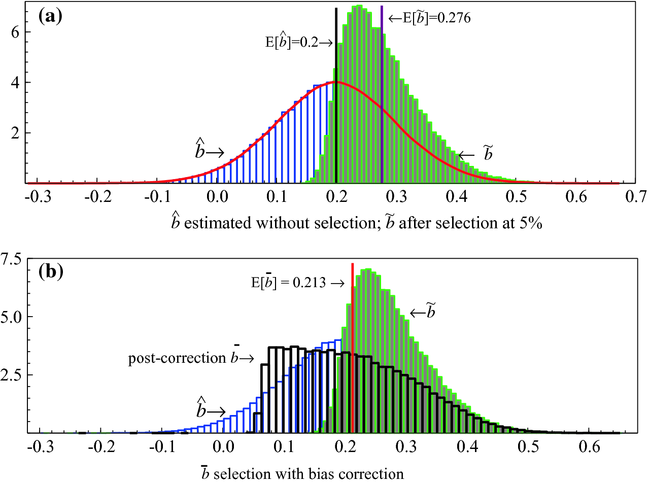
(a) The impact on the statistical distributions of selecting only significant parameters; (b) distributions after bias correction
A more important issue is that omitting relevant variables will bias the remaining retained coefficients (except if all variables are mutually orthogonal), and that effect will often be far larger than selection biases, and cannot be corrected as it is not known which omitted variables are relevant. Of course, simply asserting a relation and estimating it without selection is likely to be even more prone to such biases unless an investigator is omniscient. In almost every observational discipline, especially those facing non-stationary data, selection is inevitable. Consequently, the least-worst route is to allow for as many potentially relevant explanatory variables as feasible to avoid omitted-variables biases, and use an automatic selection approach, aka a machine-learning algorithm, balancing the costs of over and under inclusion. Hence, Campos et al. (2005) focus on methods that commence from the most general feasible specification and conduct simplification searches leading to three generations of automatic selection algorithms in the sequence Hoover and Perez (1999), PcGets by Hendry and Krolzig (2001) and Autometrics by Doornik (2009), embedded in the approach to model discovery by Hendry and Doornik (2014). We now consider the prevalence of non-stationarity in observational data.

Open Access This chapter is licensed under the terms of the Creative Commons Attribution 4.0 International License (http://creativecommons.org/licenses/by/4.0/), which permits use, sharing, adaptation, distribution and reproduction in any medium or format, as long as you give appropriate credit to the original author(s) and the source, provide a link to the Creative Commons license and indicate if changes were made.
The images or other third party material in this chapter are included in the chapter's Creative Commons license, unless indicated otherwise in a credit line to the material. If material is not included in the chapter's Creative Commons license and your intended use is not permitted by statutory regulation or exceeds the permitted use, you will need to obtain permission directly from the copyright holder.