
Discrete probability distributions can’t handle every situation.
So far we’ve looked at probability distributions where we’ve been able to specify exact values, but this isn’t the case for every set of data. Some types of data just don’t fit the probability distributions we’ve encountered so far. In this chapter, we’ll take a look at how continuous probability distributions work, and introduce you to one of the most important probability distributions in town—the normal distribution.
So far we’ve looked at probability distributions where the data is discrete. By this we mean the data is composed of distinct numeric values, and we’re been able to calculate the probability of each of these values. As an example, when we looked at the probability distribution for the winnings on a slot machine, the possible amounts we could win on each game were very precise. We knew exactly what amounts of money we could win, and we knew we’d win one of them.
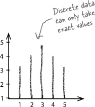
If data is discrete, it’s numeric and can take only exact values. It’s often data that can be counted in some way, such as the number of gumballs in a gumball machine, the number of questions answered correctly in a game show, or the number of breakdowns in a particular period.

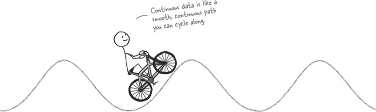
It’s not always possible to say what all the values should be in a set of data. Sometimes data covers a range, where any value within that range is possible. As an example, suppose you were asked to accurately measure pieces of string that are between 10 inches and 11 inches long. You could have measurements of 10 inches, 10.1 inches, 10.01 inches, and so on, as the length could be anything within that range.
Numeric data like this is called continuous. It’s frequently data that is measured in some way rather than counted, and a lot depends on the degree of precision you need to measure to.


The type of data you have affects how you find probabilities.
So far we’ve only looked at probability distributions that deal with discrete data. Using these probability distributions, we’ve been able to find the probabilities of exact discrete values.
The problem is that a lot of real-world problems involve continuous data, and discrete probability distributions just don’t work with this sort of data. To find probabilities for continuous data, you need to know about continuous data and continuous probability distributions.
Meanwhile, someone has a problem...
Julie is a student, and her best friend keeps trying to get her fixed up on blind dates in the hope that she’ll find that special someone. The only trouble is that not many of her dates are punctual—or indeed turn up.
Julie hates waiting alone for her date to arrive, so she’s made herself a rule: if her date hasn’t turned up after 20 minutes, then she leaves.

Here’s a sketch of the frequency showing the amount of time Julie spends waiting for her date to arrive:
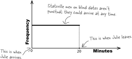
We need to find the probability that Julie will have to wait for more than 5 minutes for her date to turn up. The trouble is, the amount of time Julie has to wait is continuous data, which means the probability distributions we’ve learned thus far don’t apply.
When we were dealing with discrete data, we were able to produce a specific probability distribution. We could do this by either showing the probability of each value in a table, or by specifying whether it followed a defined probability distribution, such as the binomial or Poisson distribution. By doing this, we were able to specify the probability of each possible value. As an example, when we found the probability distribution for the winnings per game for one of Fat Dan’s slot machines, we knew all of the possible values for the winnings and could calculate the probability of each one..
x | -1 | 4 | 9 | 14 | 19 |
P(X = x) | 0.977 | 0.008 | 0.008 | 0.006 | 0.001 |
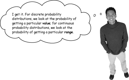
For continuous data, it’s a different matter. We can no longer give the probability of each value because it’s impossible to say what each of these precise values is. As an example, Julie’s date might turn up after 4 minutes, 4 minutes 10 seconds, or 4 minutes 10.5 seconds. Counting the number of possible options would be impossible. Instead, we need to focus on a particular level of accuracy and the probability of getting a range of values.
We can describe the probability distribution of a continuous random variable using a probability density function.
A probability density function f(x) is a function that you can use to find the probabilities of a continuous variable across a range of values. It tells us what the shape of the probability distribution is.
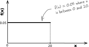
Here’s a sketch of the probability density function for the amount of time Julie spends waiting for her date to turn up:
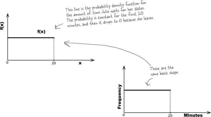
Can you see how it matches the shape of the frequency? This isn’t just a coincidence.
Probability is all about how likely things are to happen, and the frequency tells you how often values occur. The higher the relative frequency, the higher the probability of that value occurring. As the frequency for the amount of time Julie has to wait is constant across the 20 minute period, this means that the probability density function is constant too.

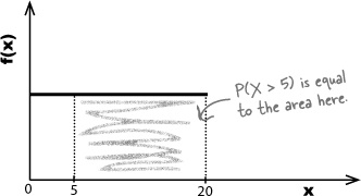
For continuous random variables, probabilities are given by area. To find the probability of getting a particular range of values, we start off by sketching the probability density function. The probability of getting a particular range of values is given by the area under the line between those values.
As an example, we want to find the probability that Julie has to wait for between 5 and 20 minutes for her date to turn up. We can find this probability by sketching the probability density function, and then working out the area under it where x is between 5 and 20.
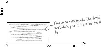
The total area under the line must be equal to 1, as the total area represents the total probability. This is because for any probability distribution, the total probability must be equal to 1, and, therefore, the area must be too.
Let’s use this to help us find the probability that Julie will need to wait for over 5 minutes for her date to arrive.
Before we can find probabilities for Julie, we need to find f(x), the probability density function.
So far, we know that f(x) is a constant value, and we know that the total area under it must be equal to 1. If you look at the sketch of f(x), the area under it forms a rectangle where the width of the base is 20. If we can find the height of the rectangle, we’ll have the value of f(x).
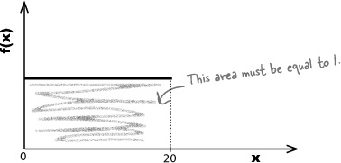
We find the area of a rectangle by multiplying its width and height together. This means that
1 | = | 20 × height |
height | = | 1/20 |
= | 0.05 |
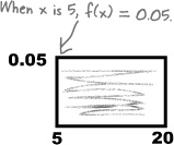
This means that f(x) must be equal to 0.05, as that ensures the total area under it will be 1. In other words,
f(x) = 0.05 | where x between 0 and 20 |
Here’s a sketch:
Now that we’ve found the probability density function, we can find P(X > 5).
The area under the probability density line between 5 and 20 is a rectangle. This means that calculating the area of this rectangle will give us the probability P(X > 5).
P(X > 5) | = | (20 – 5) × 0.05 |
= | 0.75 |
So the probability that Julie will have to wait for more than 5 minutes is 0.75.

That doesn’t work for continuous probabilities.
For continuous probabilities, we have to find the probability by calculating the area under the probability density line.
We can’t add together the probability of getting each value within the range as there are an infinite number of values. It would take forever.
The only way we can find the probability for continuous probability distributions is to work out the area underneath the curve formed by the probability density function.
When dealing with continuous data, you calculate probabilities for a range of values.
Be the Probability Density Function Solution
A bunch of probability density functions have lost track of their probabilities. Your job is to play like you’re the probability density function and work out the probability between the specified ranges. Draw a sketch if you think that will help.
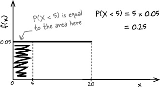
f(x) = 0.05 where 0 < x < 20
Find P(X < 5)
f(x) = 1 where 0 < x < 1
Find P(X < 0.5)
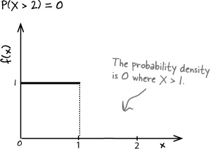
f(x) = 1 where 0 < x < 1
Find P(X > 2)
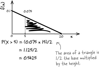
f(x) = 0.1 – 0.005x where 0 < x < 20
Find P(X > 5)

So far, we’ve looked at how you can use probability density functions to find probabilities for continuous data. We’ve found that the probability that Julie will have to wait for more than 5 minutes for her date to turn up is 0.75.

As well as preferring men who are punctual, Julie has preconceived ideas about what the love of her like should be like.

Julie loves wearing high-heeled shoes, and the higher the heel, the happier she is. The only problem is that she insists that her dates should be taller than her when she’s wearing her most extreme set of heels, and she’s running out of suitable men.
Unfortunately, the last couple of times Julie was sent on a blind date, the guys fell short of her expectations. She’s wondering how many men out there are taller than her and what the probability is that her dates will be tall enough for her high standards.
So how can we work out the probability this time?
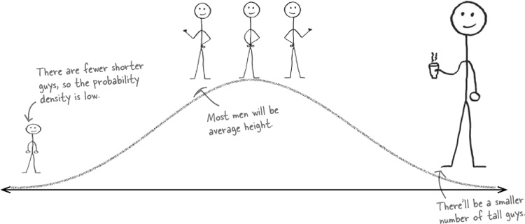
So far we’ve looked at very simple continuous distributions, but it’s unlikely these will model the heights of the men Julie might be dating. It’s likely we’ll have several men who are quite a bit shorter than average, a few really tall ones, and a lot of men somewhere in between. We can expect most of the men to be average height.

Given this pattern, the probability density of the height of the men is likely to look something like this.
This shape of distribution is actually fairly common and can be applied to lots of situations. It’s called the normal distribution.
The normal distribution is called normal because it’s seen as an ideal. It’s what you’d “normally” expect to see in real life for a lot of continuous data such as measurements.
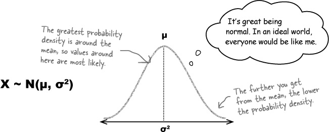
The normal distribution is in the shape of a bell curve. The curve is symmetrical, with the highest probability density in the center of the curve. The probability density decreases the further away you get from the mean. Both the mean and median are at the center and have the highest probability density.
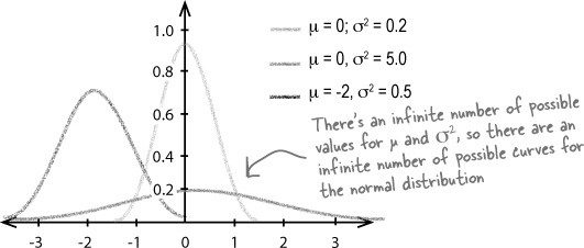
The normal distribution is defined by two parameters, μ and σ2. μ tells you where the center of the curve is, and σ gives you the spread. If a continuous random variable X follows a normal distribution with mean μ and standard deviation σ, this is generally written X ~ N(μ, σ2).
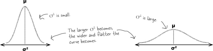
So what effect do μ and σ really have on the shape of the normal distribution?
We said that μ tells you where the center of the curve is, and σ2 indicates the spread of values. In practice, this means that as σ2 gets larger, the flatter and wider the normal curve becomes.
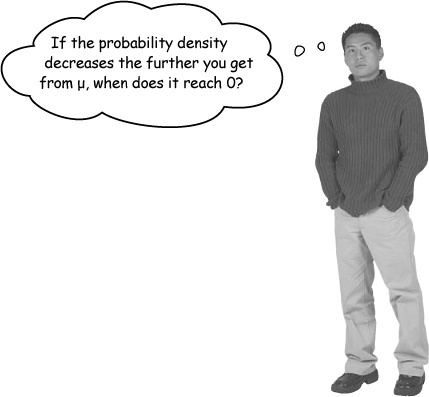
No matter how far you go out on the graph, the probability density never equals 0.
The probability density gets closer and closer to 0, but never quite reaches it. If you looked at the probability density curve a very long way from μ, you’d find that the curve just skims above 0.
Another way of looking at this is that events become more and more unlikely to occur, but there’s always a tiny chance they might.
As with any other continuous probability distribution, you find probabilities by calculating the area under the curve of the distribution. The curve gives the probability density, and the probability is given by the area between particular ranges. If, for instance, you wanted to find the probability that a variable X lies between a and b, you’d need to find the area under the curve between points a and b.
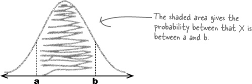
Sound complicated? Don’t worry, it’s easier than you might think.
Working out the area under the normal curve would be difficult if you had to do it all by yourself, but fortunately you have a helping hand in the form of probability tables. All you need to do is work out the range of the area you want to find, and then look up the corresponding probability in the table.
There are a few steps you need to take in order to find normal probabilities. We’ll guide you through the process, but for now here’s a roadmap of where we’re headed.
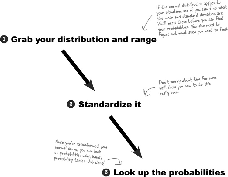
The first thing we need to do is determine the distribution of the data.
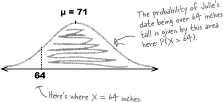
Julie has been given the mean and standard deviation of the heights of eligible men in Statsville. The mean is 71 inches, and the variance is 20.25 inches. This means that if X represents the heights of the men, X ~ N(71, 20.25).
Note
This is shorthand for “The variable X follows a normal distribution, and has a mean of 71 and a variance of 20.25.”

We also need to know which range of values will give us the right probability area. In this case, we need to find the probability that Julie’s blind date will be sufficiently tall.

Julie is 64 inches tall, so we’ll find the probability that her date is taller. Here’s a sketch:
The next step is to standardize our variable X so that the mean becomes 0 and the standard deviation 1. This gives us a standardized normal variable Z where Z ~ N(0, 1).

Probability tables only give probabilities for N(0, 1).
Probability tables focus on giving the probabilities for N(0, 1) distributions, as it would be impossible to produce probability tables for every single normal distribution curve. There are an infinite number of possible values for μ and σ2, and as the normal curve uses these as parameters to indicate the center and spread of the curve, there are also an infinite number of possible normal distribution curves.
Being able to use a standard normal distribution means that we can use the same set of probability tables for all possible values of μ and σ2. There’s just one question—how do we convert out normal distribution into a standard form?
Let’s start off by transforming our normal distribution so that the mean becomes 0 rather than 71. To do this, we move the curve to the left by 71.
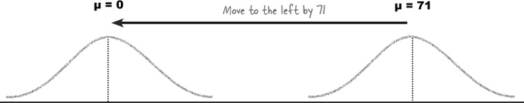
This gives us a new distribution of
X – 71 ~ N(0, 20.25)
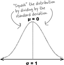
We also need to adjust the variance. To do this, we “squash” our distribution by dividing by the standard deviation. We know the variance is 20.25, so the standard deviation is 4.5.
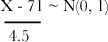
or Z ~ N(0, 1) where

Look familiar? This is the standard score we encountered when we first looked at the standard deviation in Chapter 3. In general, you can find the standard score for any normal variable X using
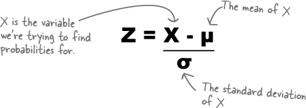
So far we’ve looked at how our probability distribution can be standardized to get from X ~ N(μ, σ2) to Z ~ N(0, 1). What we’re most interested in is actual probabilities. What we need to do is take the range of values we want to find probabilities for, and find the standard score of the limit of this range. Then we can look up the probability for our standard score using normal probability tables.
In our situation, we want to find the probability that Julie’s date is taller than her. Since Julie is 64 inches tall, we need to find P(X > 64). The limit of this range is 64, so if we calculate the standard score z of 64, we’ll be able to use this to find our probability.

Let’s find the standard score of 64.
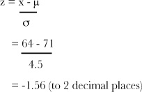
So -1.56 is the standard score of 64, using the mean and standard deviation of the men’s heights in Statsville.
Now that we have this, we can move onto the final step, using tables to look up the probability.

Sharpen your pencil Solution
It’s time to standardize. We’ll give you a distribution and value, and you have to tell us what the standard score is.
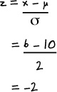
N(10, 4), value 6
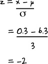
N(6.3, 9), value 0.3
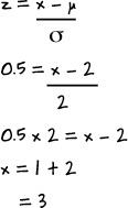
N(2, 4). If the standard score is 0.5, what’s the value?
This is the reverse of previous problems. We’re given the standard score, and we have to find the original value. We can do this by substituting in the values we know, and finding x.
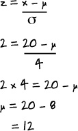
The standard score of value 20 is 2. If the variance is 16, what’s the mean?
This is a similar problem to question 3. We have to substitute in the values we know to find μ.

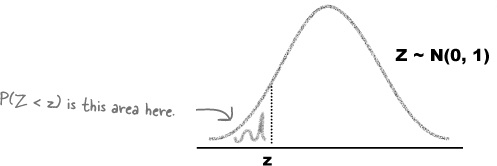
Now that we have a standard score, we can use probability tables to find our probability. Standard normal probability tables allow you to look up any value z, and then read off the corresponding probability P(Z < z).
Relax
We’ve put all the probability tables you need in Appendix B of the book.
Just flip to #1. Standard normal probabilities for the normal distribution tables you need to find probabilities in this chapter.
Start off by calculating z to 2 decimal places. This is the value that you will need to look up in the table.
To look up the probability, you need to use the first column and the top row to find your value of z. The first column gives the value of z to 1 decimal place (without rounding), and the top row gives the second decimal place. The probability is where the two intersect.
As an example, if you wanted to find P(Z < –3.27), you’d find –3.2 in the first column, .07 in the top row, and read off a probability of 0.0005.

Let’s go back to our problem with Julie. We want to find P(Z > -1.56), so let’s look up -1.56 in the probability table and see what this gives us.

So, looking up the value of –1.56 in the probability table gives us a probability of 0.0594. In other words, P(Z < –1.56) = 0.0594. This means that
P(Z > –1.56) | = | 1 – P(Z < –1.56) |
= | 1 – 0.0594 | |
= | 0.9406 |
In other words, the probability that Julie’s date is taller than her is 0.9406.

Probability Tables Up Close
Probability tables allow you to look up the probability P(Z < z) where z is some value. The problem is you don’t always want to find this sort of probability; sometimes you want to find the probability that a continuous random variable is greater than z, or between two values. How can you use probability tables to find the probability you need?
The big trick is to find a way of using the probability tables to get to what you want, usually by finding a whole area and then subtracting what you don’t need.

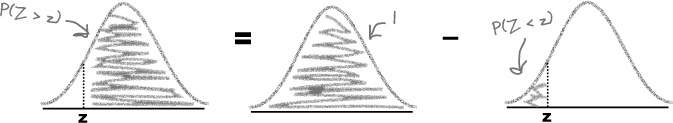
Finding P(Z > z)
We can find probabilities of the form P(Z > z) using
P(Z > z) = 1 – P(Z < z)
In other words, take the area where Z < z away from the total probability.
Finding P(a < Z < b)
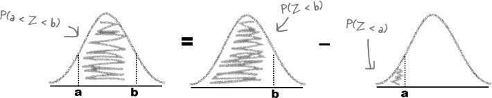
Finding this sort of probability is slightly more complicated to calculate, but it’s still possible. You can calculate this sort of probability using
Note
You could use this to find the probability that the height of Julie’s date is within a particular range.
P(a < Z < b) = P(Z < b) – P(Z < a)
In other words, calculate P(Z < b), and take away the area for P(Z < a).
Sharpen your pencil Solution
It’s time to put your probability table skills to the challenge. See if you can solve the following probability problems.
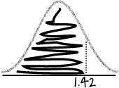
P(Z < 1.42)
We can find this probability by looking up 1.42 in the probability tables. This gives us
P(Z < 1.42) = 0.9222
P(–0.15 < Z < 0.5)
For this one, look up P(Z < 0.5), and subtract P(Z < –0.15)
P(–0.15 < Z < 0.5
P(Z < 0.5) – P(Z < –0.15)
= 0.6915 – 0.4404
= 0.2511
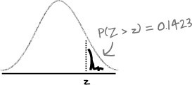
P(Z > z) = 0.1423. What’s z?
This is a slightly different problem. We’re given the probability, and need to find the value of z.
We know that P(Z > z) = 0.1423, which means that
P(Z < z)
= 1 – 0.1423
= 0.8577
The next thing to do is find which value of z has a probability of 0.8577. Looking this up in the probability tables gives us
z = 1.07
so
P(Z > 1.07) = 0.1423

Exercise
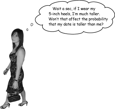
Julie has a problem. When we calculated the probability of her date being taller than her, we failed to take her high heels into account. See if you can find the probability of Julie’s date being taller than her while she’s wearing shoes with 5 inch heels.
As a reminder, Julie is 64 inches tall and X ~ N(71, 20.25) where X is the height of men in Statsville.
Exercise Solution
Julie has a problem. When we calculated the probability of her date being taller than her, we failed to take her high heels into account. See if you can find the probability of Julie’s date being taller than her while she’s wearing shoes with 5 inch heels.
As a reminder, Julie is 64 inches tall and X ~ N(71, 20.25) where X is the height of men in Statsville.
When Julie is wearing 5 inch high heels, her height is 69 inches. We need to find P(X > 69).
We need to start by finding the standard score of 178 so that we can use probability tables to look up the probabilities.
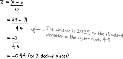
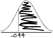
Now we’ve found z, we need to find P(Z > z) i.e. P(Z > –0.44)
P(Z > –0.44) | = 1 – P(Z < –0.44) |
= 1 – 0.3300 | |
= 0.67 |
So the probability that Julie’s date is taler than her when she’s wearing shoes with a 5 inch heel is 0.67.

Five Minute Mystery Solution
The Case of the Missing Parameters: Solved
How can Will find the mean and standard deviation?
Will can use probability tables and standard scores to get expressions for the mean and standard deviation that he can then solve.
First of all, we know that P(X < 5) = 0.0045. From probability tables, P(X < z1) where z1 = -2.61, which means that the standard score of 5 is -2.61. If we put this into the standard score formula, we get

Similarly, P(X < 15) = 0.9641, which means that the standard score of 15 is 1.8. This gives us

This gives us two equations we can solve to find μ and σ.
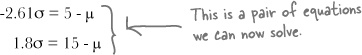
If we subtract the first equation from the second, we get
1.8σ + 2.61σ = | 15 – μ – 5 + μ |
4.41σ = | 10 |
σ = | 2.27 |
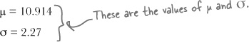
If we then substitute this into the second equation, we get
1.8 × 2.27 | = 15 – μ |
λ | = 15 – 4.086 |
= 10.914 |
In other words,
Just as the odds predicted, Julie’s latest blind date was a success! Julie had to make sure her intended soulmate was compatible with her shoes, so she made sure she wore her highest heels to put him to the test. What’s more, he was already at the venue when she arrived, so she didn’t have to wait around.

Keep reading and we’ll show you more things you can do with the normal distribution. You’ve only just scratched the surface of what you can do.
Bullet Points
The normal distribution forms the shape of a symmetrical bell curve. It’s defined using N(μ, σ2).
To find normal probabilities, start by identifying the probability range you need. Then find the standard score for the limit of this range using
You find normal probabilities by looking up your standard score in probability tables. Probability tables give you the probability of getting this value or lower.
