Random Variables

Abstract

Random variables are quantities whose value is determined by the outcome of an experiment. This chapter introduces two types of random variables: discrete and continuous, and studies a variety of such of each type. The important idea of the expected value of a random variable is introduced.

Keywords

Discrete Random Variables; Continuous Random Variables; Binomial Random Variable; Poisson Random Variable; Geometric Random Variable; Uniform Random Variable; Exponential Random Variable; Expected Value; Variance; Joint Distributions

2.1 Random Variables

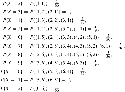
It frequently occurs that in performing an experiment we are mainly interested in some functions of the outcome as opposed to the outcome itself. For instance, in tossing dice we are often interested in the sum of the two dice and are not really concerned about the actual outcome. That is, we may be interested in knowing that the sum is seven and not be concerned over whether the actual outcome was (1, 6) or (2, 5) or (3, 4) or (4, 3) or (5, 2) or (6, 1). These quantities of interest, or more formally, these real-valued functions defined on the sample space, are known as random variables.

Since the value of a random variable is determined by the outcome of the experiment, we may assign probabilities to the possible values of the random variable.

Example 2.1

Letting X denote the random variable that is defined as the sum of two fair dice; then

P{X=2}=P{(1,1)}=136,P{X=3}=P{(1,2),(2,1)}=236,P{X=4}=P{(1,3),(2,2),(3,1)}=336,P{X=5}=P{(1,4),(2,3),(3,2),(4,1)}=436,P{X=6}=P{(1,5),(2,4),(3,3),(4,2),(5,1)}=536,P{X=7}=P{(1,6),(2,5),(3,4),(4,3),(5,2),(6,1)}=636,P{X=8}=P{(2,6),(3,5),(4,4),(5,3),(6,2)}=536,P{X=9}=P{(3,6),(4,5),(5,4),(6,3)}=436,P{X=10}=P{(4,6),(5,5),(6,4)}=336,P{X=11}=P{(5,6),(6,5)}=236,P{X=12}=P{(6,6)}=136 (2.1)

(2.1)

In other words, the random variable X can take on any integral value between two and twelve, and the probability that it takes on each value is given by Equation (2.1). Since X must take on one of the values two through twelve, we must have

1=P⋃n=212{X=n}=∑n=212P{X=n}

which may be checked from Equation (2.1). ■

Example 2.2

For a second example, suppose that our experiment consists of tossing two fair coins. Letting Y denote the number of heads appearing, then Y is a random variable taking on one of the values 0, 1, 2 with respective probabilities

P{Y=0}=P{(T,T)}=14,P{Y=1}=P{(T,H),(H,T)}=24,P{Y=2}=P{(H,H)}=14

Of course, P{Y=0}+P{Y=1}+P{Y=2}=1. ■

Example 2.3

Suppose that we toss a coin having a probability p of coming up heads, until the first head appears. Letting N denote the number of flips required, then assuming that the outcome of successive flips are independent, N is a random variable taking on one of the values 1,2,3,…, with respective probabilities

P{N=1}=P{H}=p,P{N=2}=P{(T,H)}=(1-p)p,P{N=3}=P{(T,T,H)}=(1-p)2p,⋮P{N=n}=P{(T,T,…,T︸n-1,H)}=(1-p)n-1p,n≥1

As a check, note that

P⋃n=1∞{N=n}=∑n=1∞P{N=n}=p∑n=1∞(1-p)n-1=p1-(1-p)=1■

Example 2.4

Suppose that our experiment consists of seeing how long a battery can operate before wearing down. Suppose also that we are not primarily interested in the actual lifetime of the battery but are concerned only about whether or not the battery lasts at least two years. In this case, we may define the random variable I by

I=1,ifthelifetimeofbatteryistwoormoreyears0,otherwise

If E denotes the event that the battery lasts two or more years, then the random variable I is known as the indicator random variable for event E. (Note that I equals 1 or 0 depending on whether or not E occurs.) ■

Example 2.5

Suppose that independent trials, each of which results in any of m possible outcomes with respective probabilities p1,…,pm,∑i=1mpi=1, are continually performed. Let X denote the number of trials needed until each outcome has occurred at least once.

Rather than directly considering P{X=n} we will first determine P{X>n}, the probability that at least one of the outcomes has not yet occurred after n trials. Letting Ai denote the event that outcome i has not yet occurred after the first n trials, i=1,…,m, then

P{X>n}=P⋃i=1mAi=∑i=1mP(Ai)-∑∑i<jP(AiAj)+∑∑∑i<j<kP(AiAjAk)-⋯+(-1)m+1P(A1⋯Am)

Now, P(Ai) is the probability that each of the first n trials results in a non-i outcome, and so by independence

P(Ai)=(1-pi)n

Similarly, P(AiAj) is the probability that the first n trials all result in a non-i and non-j outcome, and so

P(AiAj)=(1-pi-pj)n

As all of the other probabilities are similar, we see that

P{X>n}=∑i=1m(1-pi)n-∑∑i<j(1-pi-pj)n+∑∑∑i<j<k(1-pi-pj-pk)n-⋯

Since P{X=n}=P{X>n-1}-P{X>n}, we see, upon using the algebraic identity (1-a)n-1-(1-a)n=a(1-a)n-1, that

P{X=n}=∑i=1mpi(1-pi)n-1-∑∑i<j(pi+pj)(1-pi-pj)n-1+∑∑∑i<j<k(pi+pj+pk)(1-pi-pj-pk)n-1-⋯■

In all of the preceding examples, the random variables of interest took on either a finite or a countable number of possible values.* Such random variables are called discrete. However, there also exist random variables that take on a continuum of possible values. These are known as continuous random variables. One example is the random variable denoting the lifetime of a car, when the car’s lifetime is assumed to take on any value in some interval (a,b).

The cumulative distribution function (cdf) (or more simply the distribution function) F(·) of the random variable X is defined for any real number b,-∞<b<∞, by

F(b)=P{X≤b}

In words, F(b) denotes the probability that the random variable X takes on a value that is less than or equal to b. Some properties of the cdf F are

(i) F(b) is a nondecreasing function of b,

(ii) limb→∞F(b)=F(∞)=1,

(iii) limb→-∞F(b)=F(-∞)=0.

Property (i) follows since for a<b the event {X≤a} is contained in the event {X≤b}, and so it must have a smaller probability. Properties (ii) and (iii) follow since X must take on some finite value.

All probability questions about X can be answered in terms of the cdf F(·). For example,

P{a<X≤b}=F(b)-F(a)foralla<b

This follows since we may calculate P{a<X≤b} by first computing the probability that X≤b (that is, F(b)) and then subtracting from this the probability that X≤a (that is, F(a)).

If we desire the probability that X is strictly smaller than b, we may calculate this probability by

P{X<b}=limh→0+P{X≤b-h}=limh→0+F(b-h)

where limh→0+ means that we are taking the limit as h decreases to 0. Note that P{X<b} does not necessarily equal F(b) since F(b) also includes the probability that X equals b.

2.2 Discrete Random Variables

As was previously mentioned, a random variable that can take on at most a countable number of possible values is said to be discrete. For a discrete random variable X, we define the probability mass function p(a) of X by

p(a)=P{X=a}

The probability mass function p(a) is positive for at most a countable number of values of a. That is, if X must assume one of the values x1,x2,… then

p(xi)>0,i=1,2,…p(x)=0,allothervaluesofx

Since X must take on one of the values xi, we have

∑i=1∞p(xi)=1

The cumulative distribution function F can be expressed in terms of p(a) by

F(a)=∑allxi≤ap(xi)

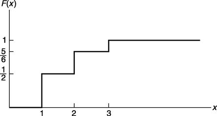
For instance, suppose X has a probability mass function given by

p(1)=12,p(2)=13,p(3)=16

then, the cumulative distribution function F of X is given by

F(a)=0,a<112,1≤a<256,2≤a<31,3≤a

This is graphically presented in Figure 2.1.

Figure 2.1 Graph of F(x).

Discrete random variables are often classified according to their probability mass functions. We now consider some of these random variables.

2.2.1 The Bernoulli Random Variable

Suppose that a trial, or an experiment, whose outcome can be classified as either a “success” or as a “failure” is performed. If we let X equal 1 if the outcome is a success and 0 if it is a failure, then the probability mass function of X is given by

p(0)=P{X=0}=1-p,p(1)=P{X=1}=p (2.2)

(2.2)

where p,0≤p≤1, is the probability that the trial is a “success.”

A random variable X is said to be a Bernoulli random variable if its probability mass function is given by Equation (2.2) for some p∈(0,1).

2.2.2 The Binomial Random Variable

Suppose that n independent trials, each of which results in a “success” with probability p and in a “failure” with probability 1-p, are to be performed. If X represents the number of successes that occur in the n trials, then X is said to be a binomial random variable with parameters (n,p).

The probability mass function of a binomial random variable having parameters (n,p) is given by

p(i)=nipi(1-p)n-i,i=0,1,…,n (2.3)

(2.3)

where

ni=n!(n-i)!i!

equals the number of different groups of i objects that can be chosen from a set of n objects. The validity of Equation (2.3) may be verified by first noting that the probability of any particular sequence of the n outcomes containing i successes and n-i failures is, by the assumed independence of trials, pi(1-p)n-i. Equation (2.3) then follows since there are ni different sequences of the n outcomes leading to i successes and n-i failures. For instance, if n=3,i=2, then there are 32=3 ways in which the three trials can result in two successes. Namely, any one of the three outcomes (s,s,f),(s,f,s),(f,s,s), where the outcome (s,s,f) means that the first two trials are successes and the third a failure. Since each of the three outcomes (s,s,f),(s,f,s),(f,s,s) has a probability p2(1-p) of occurring the desired probability is thus 32p2(1-p).

Note that, by the binomial theorem, the probabilities sum to one, that is,

∑i=0∞p(i)=∑i=0nnipi(1-p)n-i=p+(1-p)n=1

Example 2.6

Four fair coins are flipped. If the outcomes are assumed independent, what is the probability that two heads and two tails are obtained?

Solution: Letting X equal the number of heads (“successes”) that appear, then X is a binomial random variable with parameters (n=4, p=12). Hence, by Equation (2.3),

P{X=2}=42122122=38■

Example 2.7

It is known that any item produced by a certain machine will be defective with probability 0.1, independently of any other item. What is the probability that in a sample of three items, at most one will be defective?

Solution: If X is the number of defective items in the sample, then X is a binomial random variable with parameters (3, 0.1). Hence, the desired probability is given by

P{X=0}+P{X=1}=30(0.1)0(0.9)3+31(0.1)1(0.9)2=0.972■

Example 2.8

Suppose that an airplane engine will fail, when in flight, with probability 1-p independently from engine to engine; suppose that the airplane will make a successful flight if at least 50 percent of its engines remain operative. For what values of p is a four-engine plane preferable to a two-engine plane?

Solution: Because each engine is assumed to fail or function independently of what happens with the other engines, it follows that the number of engines remaining operative is a binomial random variable. Hence, the probability that a four-engine plane makes a successful flight is

42p2(1-p)2+43p3(1-p)+44p4(1-p)0=6p2(1-p)2+4p3(1-p)+p4

whereas the corresponding probability for a two-engine plane is

21p(1-p)+22p2=2p(1-p)+p2

Hence the four-engine plane is safer if

6p2(1-p)2+4p3(1-p)+p4≥2p(1-p)+p2

or equivalently if

6p(1-p)2+4p2(1-p)+p3≥2-p

which simplifies to

3p3-8p2+7p-2≥0or(p-1)2(3p-2)≥0

which is equivalent to

3p-2≥0orp≥23

Hence, the four-engine plane is safer when the engine success probability is at least as large as 23,whereas the two-engine plane is safer when this probability falls below 23. ■

Example 2.9

Suppose that a particular trait of a person (such as eye color or left handedness) is classified on the basis of one pair of genes and suppose that d represents a dominant gene and r a recessive gene. Thus a person with dd genes is pure dominance, one with rr is pure recessive, and one with rd is hybrid. The pure dominance and the hybrid are alike in appearance. Children receive one gene from each parent. If, with respect to a particular trait, two hybrid parents have a total of four children, what is the probability that exactly three of the four children have the outward appearance of the dominant gene?

Solution: If we assume that each child is equally likely to inherit either of two genes from each parent, the probabilities that the child of two hybrid parents will have dd,rr, or rd pairs of genes are, respectively, 14,14,12. Hence, because an offspring will have the outward appearance of the dominant gene if its gene pair is either dd or rd, it follows that the number of such children is binomially distributed with parameters (4,34). Thus the desired probability is

43343141=2764■

Remark on Terminology

If X is a binomial random variable with parameters (n,p), then we say that X has a binomial distribution with parameters (n,p).

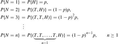
2.2.3 The Geometric Random Variable

Suppose that independent trials, each having probability p of being a success, are performed until a success occurs. If we let X be the number of trials required until the first success, then X is said to be a geometric random variable with parameter p. Its probability mass function is given by

p(n)=P{X=n}=(1-p)n-1p,n=1,2,… (2.4)

(2.4)

Equation (2.4) follows since in order for X to equal n it is necessary and sufficient that the first n-1 trials be failures and the nth trial a success. Equation (2.4) follows since the outcomes of the successive trials are assumed to be independent.

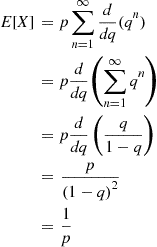
To check that p(n) is a probability mass function, we note that

∑n=1∞p(n)=p∑n=1∞(1-p)n-1=1

2.2.4 The Poisson Random Variable

A random variable X, taking on one of the values 0,1,2,…, is said to be a Poisson random variable with parameter λ, if for some λ>0,

p(i)=P{X=i}=e-λλii!,i=0,1,… (2.5)

(2.5)

Equation (2.5) defines a probability mass function since

∑i=0∞p(i)=e-λ∑i=0∞λii!=e-λeλ=1

The Poisson random variable has a wide range of applications in a diverse number of areas, as will be seen in Chapter 5.

An important property of the Poisson random variable is that it may be used to approximate a binomial random variable when the binomial parameter n is large and p is small. To see this, suppose that X is a binomial random variable with parameters (n,p), and let λ=np. Then

P{X=i}=n!(n-i)!i!pi(1-p)n-i=n!(n-i)!i!λni1-λnn-i=n(n-1)⋯(n-i+1)niλii!(1-λ/n)n(1-λ/n)i

Now, for n large and p small

1-λnn≈e-λ,n(n-1)⋯(n-i+1)ni≈1,1-λni≈1

Hence, for n large and p small,

P{X=i}≈e-λλii!

Example 2.10

Suppose that the number of typographical errors on a single page of this book has a Poisson distribution with parameter λ=1. Calculate the probability that there is at least one error on this page.

Solution:

P{X≥1}=1-P{X=0}=1-e-1≈0.633■

Example 2.11

If the number of accidents occurring on a highway each day is a Poisson random variable with parameter λ=3, what is the probability that no accidents occur today?

Solution:

P{X=0}=e-3≈0.05■

Example 2.12

Consider an experiment that consists of counting the number of α-particles given off in a one-second interval by one gram of radioactive material. If we know from past experience that, on the average, 3.2 such α-particles are given off, what is a good approximation to the probability that no more than two α-particles will appear?

Solution: If we think of the gram of radioactive material as consisting of a large number n of atoms each of which has probability 3.2/n of disintegrating and sending off an α-particle during the second considered, then we see that, to a very close approximation, the number of α-particles given off will be a Poisson random variable with parameter λ=3.2. Hence the desired probability is

P{X≤2}=e-3.2+3.2e-3.2+(3.2)22e-3.2≈0.382■

2.3 Continuous Random Variables

In this section, we shall concern ourselves with random variables whose set of possible values is uncountable. Let X be such a random variable. We say that X is a continuous random variable if there exists a nonnegative function f(x), defined for all real x∈(-∞,∞), having the property that for any set B of real numbers

P{X∈B}=∫Bf(x)dx (2.6)

(2.6)

The function f(x) is called the probability density function of the random variable X.

In words, Equation (2.6) states that the probability that X will be in B may be obtained by integrating the probability density function over the set B. Since X must assume some value, f(x) must satisfy

1=P{X∈(-∞,∞)}=∫-∞∞f(x)dx

All probability statements about X can be answered in terms of f(x). For instance, letting B=[a,b], we obtain from Equation (2.6) that

P{a≤X≤b}=∫abf(x)dx (2.7)

(2.7)

If we let a=b in the preceding, then

P{X=a}=∫aaf(x)dx=0

In words, this equation states that the probability that a continuous random variable will assume any particular value is zero.

The relationship between the cumulative distribution F(·) and the probability density f(·) is expressed by

F(a)=P{X∈(-∞,a]}=∫-∞af(x)dx

Differentiating both sides of the preceding yields

ddaF(a)=f(a)

That is, the density is the derivative of the cumulative distribution function. A somewhat more intuitive interpretation of the density function may be obtained from Equation (2.7) as follows:

Pa-ε2≤X≤a+ε2=∫a-ε/2a+ε/2f(x)dx≈εf(a)

when ε is small. In other words, the probability that X will be contained in an interval of length ε around the point a is approximately εf(a). From this, we see that f(a) is a measure of how likely it is that the random variable will be near a.

There are several important continuous random variables that appear frequently in probability theory. The remainder of this section is devoted to a study of certain of these random variables.

2.3.1 The Uniform Random Variable

A random variable is said to be uniformly distributed over the interval (0,1) if its probability density function is given by

f(x)=1,0<x<10,otherwise

Note that the preceding is a density function since f(x)≥0 and

∫-∞∞f(x)dx=∫01dx=1

Since f(x)>0 only when x∈(0,1), it follows that X must assume a value in (0,1). Also, since f(x) is constant for x∈(0,1),X is just as likely to be “near” any value in (0, 1) as any other value. To check this, note that, for any 0<a<b<1,

P{a≤X≤b}=∫abf(x)dx=b-a

In other words, the probability that X is in any particular subinterval of (0,1) equals the length of that subinterval.

In general, we say that X is a uniform random variable on the interval (α,β) if its probability density function is given by

f(x)=1β-α,ifα<x<β0,otherwise (2.8)

(2.8)

Example 2.13

Calculate the cumulative distribution function of a random variable uniformly distributed over (α,β).

Solution: Since F(a)=∫-∞af(x)dx, we obtain from Equation (2.8) that

F(a)=0,a≤αa-αβ-α,α<a<β1,a≥β■

Example 2.14

If X is uniformly distributed over (0,10), calculate the probability that (a) X<3, (b) X>7, (c) 1<X<6.

Solution:

P{X<3}=∫03dx10=310,P{X>7}=∫710dx10=310,P{1<X<6}=∫16dx10=12■

2.3.2 Exponential Random Variables

A continuous random variable whose probability density function is given, for some λ>0, by

f(x)=λe-λx,ifx≥00,ifx<0

is said to be an exponential random variable with parameter λ. These random variables will be extensively studied in Chapter 5, so we will content ourselves here with just calculating the cumulative distribution function F:

F(a)=∫0aλe-λxdx=1-e-λa,a≥0

Note that F(∞)=∫0∞λe-λxdx=1, as, of course, it must.

2.3.3 Gamma Random Variables

A continuous random variable whose density is given by

f(x)=λe-λx(λx)α-1Γ(α),ifx≥00,ifx<0

for some λ>0,α>0 is said to be a gamma random variable with parameters α,λ. The quantity Γ(α) is called the gamma function and is defined by

Γ(α)=∫0∞e-xxα-1dx

It is easy to show by induction that for integral α, say, α=n,

Γ(n)=(n-1)!

2.3.4 Normal Random Variables

We say that X is a normal random variable (or simply that X is normally distributed) with parameters μ and σ2 if the density of X is given by

f(x)=12πσe-(x-μ)2/2σ2,-∞<x<∞

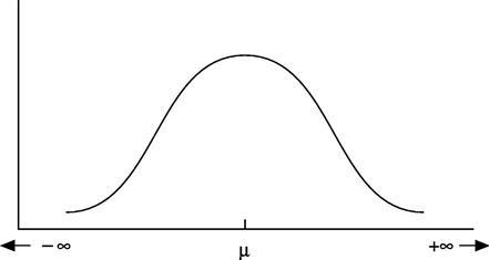
This density function is a bell-shaped curve that is symmetric around μ (see Figure 2.2).

Figure 2.2 Normal density function.

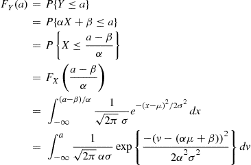
An important fact about normal random variables is that if X is normally distributed with parameters μ and σ2 then Y=αX+β is normally distributed with parameters αμ+βandα2σ2. To prove this, suppose first that α>0 and note that FY(·)*, the cumulative distribution function of the random variable Y, is given by

FY(a)=P{Y≤a}=P{αX+β≤a}=PX≤a-βα=FXa-βα=∫-∞(a-β)/α12πσe-(x-μ)2/2σ2dx=∫-∞a12πασexp-(v-(αμ+β))22α2σ2dv (2.9)

(2.9)

where the last equality is obtained by the change in variables v=αx+β. However, since FY(a)=∫-∞afY(v)dv, it follows from Equation (2.9) that the probability density function fY(·) is given by

fY(v)=12πασexp-(v-(αμ+β))22(ασ)2,-∞<v<∞

Hence, Y is normally distributed with parameters αμ+βand(ασ)2. A similar result is also true when α<0.

One implication of the preceding result is that if X is normally distributed with parameters μandσ2 then Y=(X-μ)/σ is normally distributed with parameters 0 and 1. Such a random variable Y is said to have the standard or unit normal distribution.

2.4 Expectation of a Random Variable

2.4.1 The Discrete Case

If X is a discrete random variable having a probability mass function p(x), then the expected value of X is defined by

E[X]=∑x:p(x)>0xp(x)

In other words, the expected value of X is a weighted average of the possible values that X can take on, each value being weighted by the probability that X assumes that value. For example, if the probability mass function of X is given by

p(1)=12=p(2)

then

E[X]=112+212=32

is just an ordinary average of the two possible values 1 and 2 that X can assume. On the other hand, if

p(1)=13,p(2)=23

then

E[X]=113+223=53

is a weighted average of the two possible values 1 and 2 where the value 2 is given twice as much weight as the value 1 since p(2)=2p(1).

Example 2.15

Find E[X] where X is the outcome when we roll a fair die.

Solution: Since p(1)=p(2)=p(3)=p(4)=p(5)=p(6)=16, we obtain

E[X]=116+216+316+416+516+616=72■

Example 2.16

Expectation of a Bernoulli Random Variable

Calculate E[X] when X is a Bernoulli random variable with parameter p.

Solution: Since p(0)=1-p,p(1)=p,we have

E[X]=0(1-p)+1(p)=p

Thus, the expected number of successes in a single trial is just the probability that the trial will be a success. ■

Example 2.17

Expectation of a Binomial Random Variable

Calculate E[X] when X is binomially distributed with parameters n and p.

Solution:

E[X]=∑i=0nip(i)=∑i=0ninipi(1-p)n-i=∑i=1nin!(n-i)!i!pi(1-p)n-i=∑i=1nn!(n-i)!(i-1)!pi(1-p)n-i=np∑i=1n(n-1)!(n-i)!(i-1)!pi-1(1-p)n-i=np∑k=0n-1n-1kpk(1-p)n-1-k=np[p+(1-p)]n-1=np

where the second from the last equality follows by letting k=i-1. Thus, the expected number of successes in n independent trials is n multiplied by the probability that a trial results in a success. ■

Example 2.18

Expectation of a Geometric Random Variable

Calculate the expectation of a geometric random variable having parameter p.

Solution: By Equation (2.4), we have

E[X]=∑n=1∞np(1-p)n-1=p∑n=1∞nqn-1

where q=1-p,

E[X]=p∑n=1∞ddq(qn)=pddq∑n=1∞qn=pddqq1-q=p(1-q)2=1p

In words, the expected number of independent trials we need to perform until we attain our first success equals the reciprocal of the probability that any one trial results in a success. ■

Example 2.19

Expectation of a Poisson Random Variable

Calculate E[X] if X is a Poisson random variable with parameter λ.

Solution: From Equation (2.5), we have

E[X]=∑i=0∞ie-λλii!=∑i=1∞e-λλi(i-1)!=λe-λ∑i=1∞λi-1(i-1)!=λe-λ∑k=0∞λkk!=λe-λeλ=λ

where we have used the identity ∑k=0∞λk/k!=eλ. ■

2.4.2 The Continuous Case

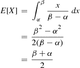
We may also define the expected value of a continuous random variable. This is done as follows. If X is a continuous random variable having a probability density function f(x), then the expected value of X is defined by

E[X]=∫-∞∞xf(x)dx

Example 2.20

Expectation of a Uniform Random Variable

Calculate the expectation of a random variable uniformly distributed over (α,β).

Solution: From Equation (2.8) we have

E[X]=∫αβxβ-αdx=β2-α22(β-α)=β+α2

In other words, the expected value of a random variable uniformly distributed over the interval (α,β) is just the midpoint of the interval. ■

Example 2.21

Expectation of an Exponential Random Variable

Let X be exponentially distributed with parameter λ. Calculate E[X].

Solution:

E[X]=∫0∞xλe-λxdx