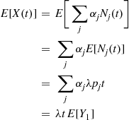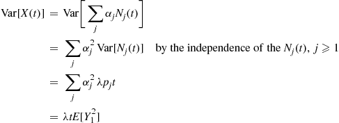
Also,

Var[X(t)]=Var∑jαjNj(t)=∑jαj2Var[Nj(t)]bytheindependenceoftheNj(t),j⩾1=∑jαj2λpjt=λtE[Y12]

where the next to last equality follows since the variance of the Poisson random variable Nj(t) is equal to its mean.

Thus, we see that the representation (5.26) results in the same expressions for the mean and variance of X(t) as were previously derived.

One of the uses of the representation (5.26) is that it enables us to conclude that as t grows large, the distribution of X(t) converges to the normal distribution. To see why, note first that it follows by the central limit theorem that the distribution of a Poisson random variable converges to a normal distribution as its mean increases. (Why is this?) Therefore, each of the random variables Nj(t) converges to a normal random variable as t increases. Because they are independent, and because the sum of independent normal random variables is also normal, it follows that X(t) also approaches a normal distribution as t increases.

Example 5.28

In Example 5.26, find the approximate probability that at least 240 people migrate to the area within the next 50 weeks.

Solution: Since λ=2,E[Yi]=5/2,E[Yi2]=43/6, we see that

E[X(50)]=250,Var[X(50)]=4300/6

Now, the desired probability is

P{X(50)⩾240}=P{X(50)⩾239.5}=PX(50)-2504300/6⩾239.5-2504300/6=1-ϕ(-0.3922)=ϕ(0.3922)=0.6525

where Table 2.3 was used to determine ϕ(0.3922), the probability that a standard normal is less than 0.3922. ■

Another useful result is that if {X(t),t⩾0} and {Y(t),t⩾0} are independent compound Poisson processes with respective Poisson parameters and distributions λ1,F1 and λ2,F2, then {X(t)+Y(t),t⩾0} is also a compound Poisson process. This is true because in this combined process events will occur according to a Poisson process with rate λ1+λ2, and each event independently will be from the first compound Poisson process with probability λ1/(λ1+λ2). Consequently, the combined process will be a compound Poisson process with Poisson parameter λ1+λ2, and with distribution function F given by

F(x)=λ1λ1+λ2F1(x)+λ2λ1+λ2F2(x)

5.4.3 Conditional or Mixed Poisson Processes

Let {N(t),t⩾0} be a counting process whose probabilities are defined as follows. There is a positive random variable L such that, conditional on L=λ, the counting process is a Poisson process with rate λ. Such a counting process is called a conditional or a mixed Poisson process.

Suppose that L is continuous with density function g. Because

P{N(t+s)-N(s)=n}=∫0∞P{N(t+s)-N(s)=n∣L=λ}g(λ)dλ=∫0∞e-λt(λt)nn!g(λ)dλ (5.27)

(5.27)

we see that a conditional Poisson process has stationary increments. However, because knowing how many events occur in an interval gives information about the possible value of L, which affects the distribution of the number of events in any other interval, it follows that a conditional Poisson process does not generally have independent increments. Consequently, a conditional Poisson process is not generally a Poisson process.

Example 5.29

If g is the gamma density with parameters m and θ,

g(λ)=θe-θλ(θλ)m-1(m-1)!,λ>0

then

P{N(t)=n}=∫0∞e-λt(λt)nn!θe-θλ(θλ)m-1(m-1)!dλ=tnθmn!(m-1)!∫0∞e-(t+θ)λλn+m-1dλ

Multiplying and dividing by (n+m-1)!(t+θ)n+m gives

P{N(t)=n}=tnθm(n+m-1)!n!(m-1)!(t+θ)n+m∫0∞(t+θ)e-(t+θ)λ((t+θ)λ)n+m-1(n+m-1)!dλ

Because (t+θ)e-(t+θ)λ((t+θ)λ)n+m-1/(n+m-1)! is the density function of a gamma (n+m,t+θ) random variable, its integral is 1, giving the result

P{N(t)=n}=n+m-1nθt+θmtt+θn

Therefore, the number of events in an interval of length t has the same distribution of the number of failures that occur before a total of m successes are amassed, when each trial is a success with probability θt+θ. ■

To compute the mean and variance of N(t), condition on L. Because, conditional on L,N(t) is Poisson with mean Lt, we obtain

E[N(t)∣L]=LtVar(N(t)∣L)=Lt

where the final equality used that the variance of a Poisson random variable is equal to its mean. Consequently, the conditional variance formula yields

Var(N(t))=E[Lt]+Var(Lt)=tE[L]+t2Var(L)

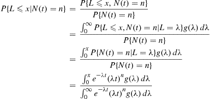
We can compute the conditional distribution function of L, given that N(t)=n, as follows.

P{L⩽x∣N(t)=n}=P{L⩽x,N(t)=n}P{N(t)=n}=∫0∞P{L⩽x,N(t)=n∣L=λ}g(λ)dλP{N(t)=n}=∫0xP{N(t)=n∣L=λ}g(λ)dλP{N(t)=n}=∫0xe-λt(λt)ng(λ)dλ∫0∞e-λt(λt)ng(λ)dλ

where the final equality used Equation (5.27). In other words, the conditional density function of L given that N(t)=n is

fL∣N(t)(λ∣n)=e-λtλng(λ)∫0∞e-λtλng(λ)dλ,λ⩾0 (5.28)

(5.28)

Example 5.30

An insurance company feels that each of its policyholders has a rating value and that a policyholder having rating value λ will make claims at times distributed according to a Poisson process with rate λ, when time is measured in years. The firm also believes that rating values vary from policyholder to policyholder, with the probability distribution of the value of a new policyholder being uniformly distributed over (0,1). Given that a policyholder has made n claims in his or her first t years, what is the conditional distribution of the time until the policyholder’s next claim?

Solution: If T is the time until the next claim, then we want to compute P{T>x∣N(t)=n}. Conditioning on the policyholder’s rating value gives, upon using Equation (5.28),

P{T>x∣N(t)=n}=∫0∞P{T>x∣L=λ,N(t)=n}×fL∣N(t)(λ∣n)dλ=∫01e-λxe-λtλndλ∫01e-λtλndλ■

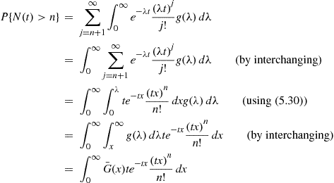
There is a nice formula for the probability that more than n events occur in an interval of length t. In deriving it we will use the identity

∑j=n+1∞e-λt(λt)jj!=∫0tλe-λx(λx)nn!dx (5.29)

(5.29)

which follows by noting that it equates the probability that the number of events by time t of a Poisson process with rate λ is greater than n with the probability that the time of the (n+1)st event of this process (which has a gamma (n+1,λ) distribution) is less than t. Interchanging λ and t in Equation (5.29) yields the equivalent identity

∑j=n+1∞e-λt(λt)jj!=∫0λte-tx(tx)nn!dx (5.30)

(5.30)

Using Equation (5.27) we now have

P{N(t)>n}=∑j=n+1∞∫0∞e-λt(λt)jj!g(λ)dλ=∫0∞∑j=n+1∞e-λt(λt)jj!g(λ)dλ(byinterchanging)=∫0∞∫0λte-tx(tx)nn!dxg(λ)dλ(using(5.30))=∫0∞∫x∞g(λ)dλte-tx(tx)nn!dx(byinterchanging)=∫0∞G¯(x)te-tx(tx)nn!dx

5.5 Random Intensity Functions and Hawkes Processes

Whereas the intensity function λ(t) of a nonhomogeneous Poisson process is a deterministic function, there are counting processes {N(t),t⩾0} whose intensity function value at time t, call it R(t), is a random variable whose value depends on the history of the process up to time t. That is, if we let Ht denote the “history” of the process up to time t then R(t), the intensity rate at time t, is a random variable whose value is determined by Ht and which is such that

P(N(t+h)-N(t)=1∣Ht)=R(t)h+o(h)

and

P(N(t+h)-N(t)⩾2∣Ht)=o(h)

The Hawkes process is an example of a counting process having a random intensity function. This counting process assumes that there is a base intensity value λ>0, and that associated with each event is a nonnegative random variable, called a mark, whose value is independent of all that has previously occurred and has distribution F. Whenever an event occurs, it is supposed that the current value of the random intensity function increases by the amount of the event’s mark, with this increase decreasing over time at an exponential rate α. More specifically, if there have been a total of N(t) events by time t, with S1<S2<…<SN(t) being the event times and Mi being the mark of event i,i=1,…,N(t), then

R(t)=λ+∑i=1N(t)Mie-α(t-Si)

In other words, a Hawkes process is a counting process in which

1. R(0)=λ;

2. whenever an event occurs, the random intensity increases by the value of the event’s mark;

3. if there are no events between s and s+t then R(s+t)=λ+(R(s)-λ)e-αt.

Because the intensity increases each time an event occurs, the Hawkes process is said to be a self-exciting process.

We will derive E[N(t)], the expected number of events of a Hawkes process that occur by time t. To do so, we will need the following lemma, which is valid for all counting processes.

Lemma

Let R(t),t⩾0 be the random intensity function of the counting process {N(t),t⩾0} having N(0)=0. Then, with m(t)=E[N(t)]

m(t)=∫0tE[R(s)]ds

Proof

E[N(t+h)∣N(t),R(t)]=N(t)+R(t)h+o(h)

Taking expectations gives

E[N(t+h)]=E[N(t)]+E[R(t)]h+o(h)

That is,

m(t+h)=m(t)+hE[R(t)]+o(h)

or

m(t+h)-m(t)h=E[R(t)]+o(h)h

Letting h go to 0 gives

m′(t)=E[R(t)]

Integrating both sides from 0 to t now gives the result:

m(t)=∫0tE[R(s)]ds■

Using the preceding, we can now prove the following proposition.

Proposition 5.5

If μ is the expected value of a mark in a Hawkes process, then for this process

E[N(t)]=λt+λμ(μ-α)2(e(μ-α)t-1-(μ-α)t)

Proof

To determine the mean value function m(t) it suffices, by the preceding lemma, to determine E[R(t)], which will be accomplished by deriving and then solving a differential equation. To begin note that, with Mt(h) equal to the sum of the marks of all events occurring between t and t+h,

R(t+h)=λ+(R(t)-λ)e-αh+Mt(h)+o(h)

Letting g(t)=E[R(t)] and taking expectations of the preceding gives

g(t+h)=λ+(g(t)-λ)e-αh+E[Mt(h)]+o(h)

Using the identity e-αh=1-αh+o(h) shows that

g(t+h)=λ+(g(t)-λ)(1-αh)+E[Mt(h)]+o(h)=g(t)-αhg(t)+λαh+E[Mt(h)]+o(h) (5.31)

(5.31)

Now, given R(t), there will be 1 event between t and t+h with probability R(t)h+o(h), and there will be 2 or more with probability o(h). Hence, conditioning on the number of events between t and t+h yields, upon using that μ is the expected value of a mark, that

E[Mt(h)∣R(t)]=μR(t)h+o(h)

Taking expectations of both sides of the preceding gives that

E[Mt(h)]=μg(t)h+o(h)