9.5 System Life as a Function of Component Lives
For a random variable having distribution function G , we define G¯(a)≡1-G(a)
 to be the probability that the random variable is greater than a
 .
.
Consider a system in which the i th component functions for a random length of time having distribution Fi
 and then fails. Once failed it remains in that state forever. Assuming that the individual component lifetimes are independent, how can we express the distribution of system lifetime as a function of the system reliability function r(p)
 and the individual component lifetime distributions Fi,i=1,…,n
 ?
?
To answer this we first note that the system will function for a length of time t or greater if and only if it is still functioning at time t
 . That is, letting F
 denote the distribution of system lifetime, we have
F¯(t)=P{systemlife>t}=P{system is functioning at timet}
But, by the definition of r(p) we have
P{system is functioning at timet}=r(P1(t),…,Pn(t))
where
Pi(t)=P{componentiis functioning att}=P{lifetimeofi>t}=F¯i(t)
Hence, we see that
F¯(t)=r(F¯1(t),…,F¯n(t)) (9.14)
 (9.14)
Example 9.20
In a series system, r(p)=∏1npi and so from Equation (9.14)
F¯(t)=∏1nF¯i(t)
which is, of course, quite obvious since for a series system the system life is equal to the minimum of the component lives and so will be greater than t if and only if all component lives are greater than t
 . ■
. ■
Example 9.21
In a parallel system r(p)=1-∏1n(1-pi) and so
F¯(t)=1-∏1nFi(t)
The preceding is also easily derived by noting that, in the case of a parallel system, the system life is equal to the maximum of the component lives. ■
For a continuous distribution G , we define λ(t)
 , the failure rate function of G
 , by
, by
λ(t)=g(t)G¯(t)
where g(t)=d/dtG(t) . In Section 5.2.2, it is shown that if G
 is the distribution of the lifetime of an item, then λ(t)
 represents the probability intensity that a t
 -year-old item will fail. We say that G
 is an increasing failure rate (IFR) distribution if λ(t)
 is an increasing function of t
 . Similarly, we say that G
 is a decreasing failure rate (DFR) distribution if λ(t)
 is a decreasing function of t
 .
.
Example 9.22
The Weibull Distribution
A random variable is said to have the Weibull distribution if its distribution is given, for some λ>0,α>0 , by
, by
G(t)=1-e-(λt)α,t⩾0
The failure rate function for a Weibull distribution equals
λ(t)=e-(λt)αα(λt)α-1λe-(λt)α=αλ(λt)α-1
Thus, the Weibull distribution is IFR when α⩾1 , and DFR when 0<α⩽1
 ; when α=1,G(t)=1-e-λt
 , the exponential distribution, which is both IFR and DFR. ■
Example 9.23
The Gamma Distribution
A random variable is said to have a gamma distribution if its density is given, for some λ>0,α>0 , by
, by
g(t)=λe-λt(λt)α-1Γ(α)fort⩾0
where
Γ(α)≡∫0∞e-ttα-1dt
For the gamma distribution,
1λ(t)=G¯(t)g(t)=∫t∞λe-λx(λx)α-1dxλe-λt(λt)α-1=∫t∞e-λ(x-t)xtα-1dx
With the change of variables u=x-t , we obtain
1λ(t)=∫0∞e-λu1+utα-1du
Hence, G is IFR when α⩾1
 and is DFR when 0<α⩽1
 . ■
. ■
Suppose that the lifetime distribution of each component in a monotone system is IFR. Does this imply that the system lifetime is also IFR? To answer this, let us at first suppose that each component has the same lifetime distribution, which we denote by G . That is, Fi(t)=G(t),i=1,…,n
 . To determine whether the system lifetime is IFR, we must compute λF(t)
 , the failure rate function of F
 . Now, by definition,
λF(t)=(d/dt)F(t)F¯(t)=(d/dt)[1-r(G¯(t))]r(G¯(t))
where
r(G¯(t))≡r(G¯(t),…,G¯(t))
Hence,
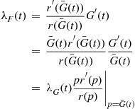
λF(t)=r′(G¯(t))r(G¯(t))G′(t)=G¯(t)r′(G¯(t))r(G¯(t))G′(t)G¯(t)=λG(t)pr′(p)r(p)p=G¯(t) (9.15)
 (9.15)
Since G¯(t) is a decreasing function of t
 , it follows from Equation (9.15) that if each component of a coherent system has the same IFR lifetime distribution, then the distribution of system lifetime will be IFR if pr′(p)/r(p)
 is a decreasing function of p
  .
.
Example 9.24
The k -out-of-n
 System with Identical Components
Consider the k -out-of-n
 system, which will function if and only if k
 or more components function. When each component has the same probability p
 of functioning, the number of functioning components will have a binomial distribution with parameters n
 and p
and p . Hence,
r(p)=∑i=knnipi(1-p)n-i
which, by continual integration by parts, can be shown to be equal to
r(p)=n!(k-1)!(n-k)!∫0pxk-1(1-x)n-kdx
Upon differentiation, we obtain
r′(p)=n!(k-1)!(n-k)!pk-1(1-p)n-k
Therefore,
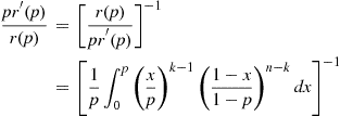
pr′(p)r(p)=r(p)pr′(p)-1=1p∫0pxpk-11-x1-pn-kdx-1
Letting y=x/p yields
pr′(p)r(p)=∫01yk-11-yp1-pn-kdy-1
Since (1-yp)/(1-p) is increasing in p
 , it follows that pr′(p)/r(p)
 is decreasing in p
 . Thus, if a k
 -out-of-n
 system is composed of independent, like components having an increasing failure rate, the system itself has an increasing failure rate. ■
It turns out, however, that for a k -out-of-n
 system, in which the independent components have different IFR lifetime distributions, the system lifetime need not be IFR. Consider the following example of a two-out-of-two (that is, a parallel) system.
Example 9.25
A Parallel System That Is Not IFR
The life distribution of a parallel system of two independent components, the i th component having an exponential distribution with mean 1/i,i=1,2
 , is given by
F¯(t)=1-(1-e-t)(1-e-2t)=e-2t+e-t-e-3t
Therefore,
λ(t)=f(t)F¯(t)=2e-2t+e-t-3e-3te-2t+e-t-e-3t
It easily follows upon differentiation that the sign of λ′(t) is determined by e-5t-e-3t+3e-4t
 , which is positive for small values and negative for large values of t
 . Therefore, λ(t)
 is initially strictly increasing, and then strictly decreasing. Hence, F
 is not IFR. ■
Remark
The result of the preceding example is quite surprising at first glance. To obtain a better feel for it we need the concept of a mixture of distribution functions. The distribution function G is said to be a mixture of the distributions G1
 and G2
 if for some p,0<p<1
 ,
,
G(x)=pG1(x)+(1-p)G2(x) (9.16)
 (9.16)
Mixtures occur when we sample from a population made up of two distinct groups. For example, suppose we have a stockpile of items of which the fraction p are type 1 and the fraction 1-p
 are type 2. Suppose that the lifetime distribution of type 1 items is G1
 and of type 2 items is G2
 . If we choose an item at random from the stockpile, then its life distribution is as given by Equation (9.16).
Consider now a mixture of two exponential distributions having rates λ1 and λ2
 where λ1<λ2
 . We are interested in determining whether or not this mixture distribution is IFR. To do so, we note that if the item selected has survived up to time t
 , then its distribution of remaining life is still a mixture of the two exponential distributions. This is so since its remaining life will still be exponential with rate λ1
 if it is type 1 or with rate λ2
 if it is a type 2 item. However, the probability that it is a type 1 item is no longer the (prior) probability p
 but is now a conditional probability given that it has survived to time t
 . In fact, its probability of being a type 1 is
P{type 1∣life>t}=P{type1,life>t}P{life>t}=pe-λ1tpe-λ1t+(1-p)e-λ2t
As the preceding is increasing in t , it follows that the larger t
 is, the more likely it is that the item in use is a type 1 (the better one, since λ1<λ2
 ). Hence, the older the item is, the less likely it is to fail, and thus the mixture of exponentials far from being IFR is, in fact, DFR.
Now, let us return to the parallel system of two exponential components having respective rates λ1 and λ2
 . The lifetime of such a system can be expressed as the sum of two independent random variables, namely,
systemlife=Exp(λ1+λ2)+Exp(λ1)withprobabilityλ2λ1+λ2Exp(λ2)withprobabilityλ1λ1+λ2
The first random variable whose distribution is exponential with rate λ1+λ2 represents the time until one of the components fails, and the second, which is a mixture of exponentials, is the additional time until the other component fails. (Why are these two random variables independent?)
Now, given that the system has survived a time t , it is very unlikely when t
 is large that both components are still functioning, but instead it is far more likely that one of the components has failed. Hence, for large t
 , the distribution of remaining life is basically a mixture of two exponentials—and so as t
 becomes even larger its failure rate should decrease (as indeed occurs). ■
Recall that the failure rate function of a distribution F(t) having density f(t)=F′(t)
 is defined by
λ(t)=f(t)1-F(t)
By integrating both sides, we obtain
∫0tλ(s)ds=∫0tf(s)1-F(s)ds=-logF¯(t)
Hence,
F¯(t)=e-Λ(t) (9.17)
 (9.17)
where
Λ(t)=∫0tλ(s)ds
The function Λ(t) is called the hazard function of the distribution F
 .
.
Definition 9.1
A distribution F is said to have increasing failure on the average (IFRA) if
Λ(t)t=∫0tλ(s)dst (9.18)
 (9.18)
increases in t for t⩾0
 .
.
In other words, Equation (9.18) states that the average failure rate up to time t increases as t
 increases. It is not difficult to show that if F
 is IFR, then F
 is IFRA; but the reverse need not be true.
Note that F is IFRA if Λ(s)/s⩽Λ(t)/t
 whenever 0⩽s⩽t
 , which is equivalent to
Λ(αt)αt⩽Λ(t)tfor0⩽α⩽1,allt⩾0
But by Equation (9.17) we see that Λ(t)=-logF¯(t) , and so the preceding is equivalent to
-logF¯(αt)⩽-αlogF¯(t)
or equivalently,
logF¯(αt)⩾logF¯α(t)
which, since log x is a monotone function of x
 , shows that F
 is IFRA if and only if
F¯(αt)⩾F¯α(t)for0⩽α⩽1,allt⩾0 (9.19)
 (9.19)
For a vector p=(p1,…,pn) we define pα=(p1α,…,pnα)
 . We shall need the following proposition.
Proposition 9.2
Any reliability function r(p) satisfies
r(pα)⩾[r(p)]α,0⩽α⩽1
Proof
We prove this by induction on n , the number of components in the system. If n=1
 , then either r(p)≡0,r(p)≡1,orr(p)≡p
 . Hence, the proposition follows in this case.
Assume that Proposition 9.2 is valid for all monotone systems of n-1 components and consider a system of n
 components having structure function ϕ
 . By conditioning upon whether or not the n
 th component is functioning, we obtain
r(pα)=pnαr(1n,pα)+(1-pnα)r(0n,pα) (9.20)
 (9.20)
Now consider a system of components 1 through n-1 having a structure function ϕ1(x)=ϕ(1n,x)
 . The reliability function for this system is given by r1(p)=r(1n,p)
 ; hence, from the induction assumption (valid for all monotone systems of n-1
 components), we have
r(1n,pα)⩾[r(1n,p)]α
Similarly, by considering the system of components 1 through n-1 and structure function ϕ0(x)=ϕ(0n,x)
 , we obtain
r(0n,pα)⩾[r(0n,p)]α
Thus, from Equation (9.20), we obtain
r(pα)⩾pnα[r(1n,p)]α+(1-pnα)[r(0n,p)]α
which, by using the lemma to follow (with λ=pn,x=r(1n,p) , y=r(0n,p)
 ), implies that
r(pα)⩾[pnr(1n,p)+(1-pn)r(0n,p)]α=[r(p)]α
which proves the result. ■
Lemma 9.3
If 0⩽α⩽1,0⩽λ⩽1 , then
h(y)=λαxα+(1-λα)yα-(λx+(1-λ)y)α⩾0
for all 0⩽y⩽x .
.
Proof
The proof is left as an exercise. ■
We are now ready to prove the following important theorem.
Theorem 9.2
For a monotone system of independent components, if each component has an IFRA lifetime distribution, then the distribution of system lifetime is itself IFRA.
Proof
The distribution of system lifetime F is given by
F¯(αt)=r(F¯1(αt),…,F¯n(αt))
Hence, since r is a monotone function, and since each of the component distributions F¯i
 is IFRA, we obtain from Equation (9.19)
F¯(αt)⩾r(F¯1α(t),…,F¯nα(t))⩾[r(F¯1(t),…,F¯n(t))]α=F¯α(t)
which by Equation (9.19) proves the theorem. The last inequality followed, of course, from Proposition 9.2. ■

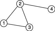

 is based on expressing the desired probability as the probability of the intersection of events. To do so, let
  denote the minimal path sets as before, and define the events,
  by
by
 (9.11)
 is down can only increase the probability that at least one component of
  is down (or else leave the probability unchanged if
  and
and  do not overlap). Hence, intuitively
 (9.12)
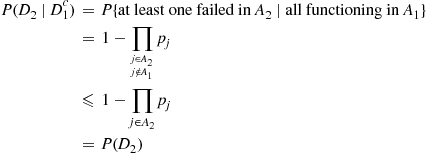


 denote the minimal cut sets and define the events
  by
by
 occur, we have
 . Hence,
 (9.13)
 if there is not too much overlap in the minimal path sets, and the lower bound to be close if there is not too much overlap in the minimal cut sets.
 , we define
  to be the probability that the random variable is greater than
  .
. th component functions for a random length of time having distribution
  and then fails. Once failed it remains in that state forever. Assuming that the individual component lifetimes are independent, how can we express the distribution of system lifetime as a function of the system reliability function
  and the individual component lifetime distributions
  ?
? or greater if and only if it is still functioning at time
  . That is, letting
  denote the distribution of system lifetime, we have
 we have

 (9.14)
 , we define
  , the failure rate function of
  , by
, by
 . In Section 5.2.2, it is shown that if
  is the distribution of the lifetime of an item, then
  represents the probability intensity that a
  -year-old item will fail. We say that
  is an increasing failure rate (IFR) distribution if
  is an increasing function of
  . Similarly, we say that
  is a decreasing failure rate (DFR) distribution if
  is a decreasing function of
  .
. . That is,
  . To determine whether the system lifetime is IFR, we must compute
  , the failure rate function of
  . Now, by definition,

 (9.15)
 is a decreasing function of
  , it follows from Equation (9.15) that if each component of a coherent system has the same IFR lifetime distribution, then the distribution of system lifetime will be IFR if
  is a decreasing function of
  .
. -out-of-
 system, in which the independent components have different IFR lifetime distributions, the system lifetime need not be IFR. Consider the following example of a two-out-of-two (that is, a parallel) system.
 having density
  is defined by

 (9.17)

 is called the hazard function of the distribution
  .
. increases as
  increases. It is not difficult to show that if
  is IFR, then
  is IFRA; but the reverse need not be true.
 is IFRA if
  whenever
  , which is equivalent to
 , and so the preceding is equivalent to

 is a monotone function of
  , shows that
  is IFRA if and only if
 (9.19)
 we define
  . We shall need the following proposition.
 and the component lifetime distributions
  .
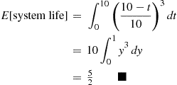
. or larger if and only if the system is still functioning at time
  , we have
 . Hence, by a well-known formula that states that for any nonnegative random variable
  ,
,
 (9.21)


