APPENDIX A
Probability
The mathematics that underly options theory can appear imposing. However, the real challenges in practical options trading and risk management are conceptual, not mathematical. I do presume some exposure to undergraduate‐level probability, statisics, and calculus. However, this appendix is written to provide a refresher on these topics via simple, example‐based explanations of the mathematical concepts in the main text for readers who may have lost familiarity with these topics over the course of time. This appendix should be sufficient to keep this textbook self‐contained.
A.1 PROBABILITY DENSITY FUNCTIONS (PDFS)
A.1.1 Discrete Random Variables and PMFs
Before studying PDFs, let us begin with probability mass functions (PMFs). PMFs provide a helpful introduction to PDFs, because they are the discrete state analogs of PDFs.
The EUR‐USD spot rate at a future time  ,
,  , is a random variable. Suppose that it can take one of three discrete values, 1.37, 1.39, and 1.41. Suppose also that the probabilities with which these values occur are
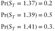
The PMF belonging to  is shown in Figure A.1. It is a plot of the probability with which EUR‐USD takes each of its possible values at
  . We have shown three states here, but we can extend this idea to many discrete states.
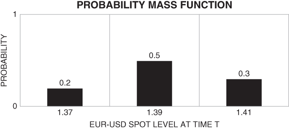
FIGURE A.1 The figure shows the PMF of  . In this case,
  can take one of three discrete values. The PMF gives us the probability that
  takes each of these values.
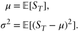
The expected value of  , denoted
  , is calculated as follows.
where  . In words, the expectation of
  is the weighted average value of
  , with the weights given by the PMF.
If we wished to extend this idea to infinitely many, or a continuum of, states, then we must turn to PDFs. This is the topic of the next subsection.
A.1.2 Continuous Random Variables and PDFs
Next, suppose that  can take a continuum of values. The probability that
  is between value
  and
and  at time
  is given by
where  is the probability density function belonging to
  . In words, there is a function
  , and the area underneath this function between
  and
and  provides the probability that
  will lie between
  and
and  . Figure A.2 and its caption explain this idea.
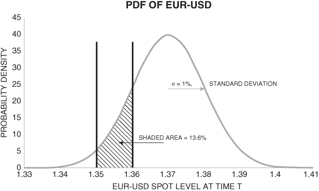
FIGURE A.2 The line shows the probability density function (of EUR‐USD spot at time  in this example),
  . Suppose we wish to calculate the probability that EUR‐USD is between
  and
and  at time
  . This is found by calculating the shaded area under the PDF,
  , which is 13.6% in our example, assuming a normal distribution with zero mean and standard deviation
  . See Section A.1.3 for more on normal distributions.
The cumulative density function, or CDF, is denoted by  and it is the probability that
  . That is,
For option contracts, spot rates are rounded to the nearest pip. Therefore, strictly speaking, they take discrete rather than continuous values. However, the reason that practitioners apply PDFs rather than PMFs in their modeling is that, quite simply, there are a lot of pips! For example, EUR‐USD is rounded to four decimal places and so to specify just the probabilities of spot landing between 1.3500 and 1.3900, the modeler would have to specify 401 bars on a chart similar to Figure A.1. It is more convenient to treat the spot rate as a continuum and then specify  . Then, if we wish to calculate the probability that EUR‐USD expires at exactly 1.3700, we can apply Equation (A.2), setting
 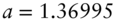 and
and  .
.
Analogous to the PMF, the expected value of  is calculated as follows,
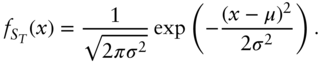
A.1.3 Normal and Log‐normal Distributions
The normal distribution has two parameters, a mean and a standard derivation, or variance. If  is normally distributed, I denote it as
Here,  is the mean of
  and
and  is its standard deviation (
 is its variance). That is,
The PDF of  is given by
 is shown in Figure A.3.
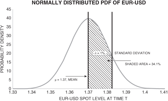
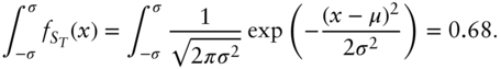
FIGURE A.3 The figure draws the function from Equation (A.3) for EUR‐USD using  and
and  . The area contained within
 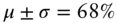 . Therefore the probability that the EUR‐USD spot rate is
  is 68%.
There are two important points to note relating to Equation (A.3). The first is that the peak of  occurs at
  . The second, is that the probability that
 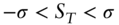 is 0.68. That is, using our result from Section A.1.2,
If  is log‐normally distributed, I denote it as
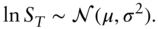
The important point to note is that  can now never be negative. Indeed, this is one of the primary reasons that the log‐normal distribution was applied in securities modeling rather than the normal distribution.
There are two important points for readers to note. First, when  is low then under the log‐normal distribution the spot price behaves in a manner very similar to the normal distribution. This is illustrated in Figure A.4. This is also the reason that the early chapters in this book explain the main concepts in options theory using normal distributions.
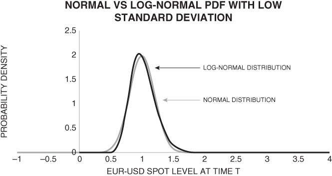
FIGURE A.4 The black line shows a log‐normal distribution and the gray line shows a normal distribution setting  and
and  . Since
  is (relatively) small, the normal distribution and log‐normal distribution are distinguishable by only a small amount.
Second, as  increases the log‐normal and normal distributions deviate, as shown in Figure A.5. The normal distribution is symmetric and therefore remains positive for negative values of the spot rate. The log‐normal distribution allows only positive values for the spot rate, and it does so by devloping a positive skewness. That is, it puts the weight that the normal distribution has in the left tail, into an extended right tail. The peak also shifts to the left.
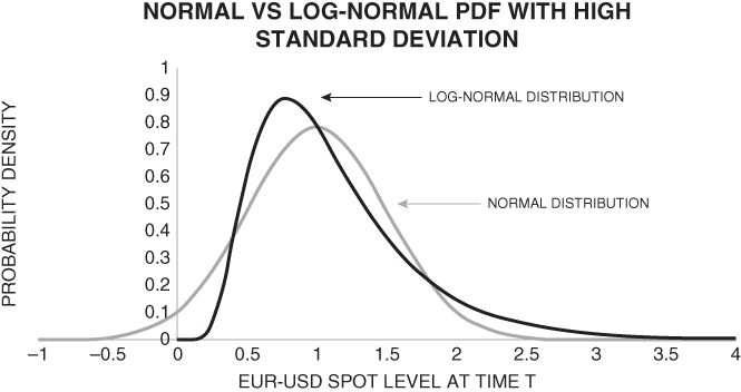
FIGURE A.5 The gray line shows the normal distribution and the black line shows a log‐normal distribution with  and
and  . Since
  is large, the lines deviate from one another. While the normal distribution remains symmetric, and remains positive for negative values of EUR‐USD spot, the log‐normal distribution develops a positive skewness and does not allow probability that EUR‐USD goes negative.