CHAPTER 11
Predictability and Mean Reversion

The majority of the ideas presented in this text rest on the idea that the spot rate is a martingale (Equation (2.9)) and it therefore exhibits no mean reversion or autocorrelation. This leads to the variance of the PDF growing with time. This growth is linear in the case of IID returns. This book has presented options theory based on this assumption. The main purpose in this chapter is to provide some empirical evidence to support this idea.

11.1 THE PAST AND THE FUTURE

Are future FX rates predictable using past rates alone? Is there mean reversion? Upon first inspection, one may be forgiven for suggesting that these questions are overly simplistic. After all, market participants are continuously bombarded with far more information relevant for forming forecasts than just past FX rates. However, this question is important and interesting at least partly because options theory is built on the idea that the discounted spot process is a martingale, although under the risk‐neutral probability measure. If the answer to the previous questions turns out to be yes, then there may exist exploitable profitable trading opportunities that take advantage of a misspecification in option pricing models. More generally, by studying this question, we learn whether the probability distributions that we use to model FX rates for the purpose of option pricing should incorporate some level of price‐based predictability.

I begin by restating the question in probabilistic terms. This will allow us to construct a statistical test to apply to a set of historical FX data. Let denote the FX rate at time and define the log return between time and by

If the relation

(11.1)

for all and holds for an arbitrary function , then past prices cannot be used to forecast future returns. The intuition here is that there must be some correlation between the past, or some function of the past, and future returns to use the past to say anything about the future. Therefore, a probabilistic statement of our question is simply, does Equation (11.1) hold in historical FX data?

To study this question, I take as a starting point the special case of (11.1) in which is a linear function. If is linear, then in effect we are testing for the existence of autocorrelations. Relation (11.1) simplifies to

(11.2)

Testing (11.2) is the topic of the next section.

11.2 EMPIRICAL ANALYSIS

The aim in this section is to test the hypothesis that Equation (11.2) holds in historical FX data. This involves two steps. The first is to estimate the quantity . This is straightforward; I replace the population moments in (11.2) with their sample counterparts.

The second step is to estimate the standard error of the estimate. The reason for this is that, even if the true autocorrelation in returns is zero, the estimated autocorrelation may not be zero.

Although the data set used in this analysis is relatively large, it is finite in size and so there may not be sufficiently many data points for the sample autocorrelation to converge to the value of its population counterpart. The standard error of the estimate provides a measure of the uncertainty associated with the autocorrelation estimate. Here, I do not reject relation (11.2) unless the estimate lies at least 1.96 standard deviations from zero. The number 1.96 is chosen because this corresponds to just a 5% chance that we reject (11.2) even if it is true. Using a number less than 1.96 would increase the chance of a false rejection, which is, of course, undesirable. Increasing this number further would decrease the chance of a rejection of (11.2) altogether. Nevertheless, the reader will see below that the implications of the statistics presented in this analysis are robust and relatively insensitive to the choice of rejection level.

Furthermore, to ensure that the results presented here are convincing, I calculate the standard errors using two separate techniques, a bootstrap method and a Generalized Method of Moments (GMM)‐based method.

The empirical analysis uses daily FX rate data for the Japanese yen (JPY), British pound (GBP), Euro (EUR), Canadian dollar (CAD), Australian dollar (AUD), and Swiss Franc (CHF) all against the US dollar (USD). Accordingly, I set and take daily returns, for . Here, denotes the data sample size. All the data samples end on 10 March 2011. However, depends on the currency pair in question because the samples start on different dates.

---

WHY STUDY RETURNS RATHER THAN EXCHANGE RATES DIRECTLY?

Most empirical work uses returns because they are plausibly stationary over time. Stationary does not mean constant. It means that the joint distribution of depends only on , and not on , and the distribution of does not depend on . The following example illustrates why this is important in empirical work. For convenience, we drop the superscript.

Suppose that our aim is to calculate the variance of returns,

To estimate the required population moments and , one would typically take a time series of historical data, , and calculate the respective sample moments, and . However, these sample moments clearly cannot converge to their population counterparts if were drawn from a distribution with a different mean and variance to , and were drawn from a distribution with yet another mean and variance, and so on; we require many samples from the same distribution. Stationarity implies each is drawn from the same distribution so that

(11.3)

(11.4)

Stationarity (and some other conditions, for which I refer the reader to Singleton, 2006) allow sample moments calculated over time to converge to their population counterparts.

Exchange rates themselves are unlikely to be stationary variables. First, their variance grows with time. One is more sure of the USD‐JPY exchange rate tomorrow than of this exchange rate in a year's time; the variance of is smaller than that of . This violates a condition analogous to (11.4) since depends on .

Second, exchange rates may tend to rise or fall with time depending on, among other things, inflation and interest rate differentials between currencies. Such a tendencies violate the analogous condition to (11.3) since depends on .

A final point to note is that stationarity forces only unconditional distribution of returns to remain unchanged over time. The conditional distribution may change.

---

The fixed exchange rate mechanism broke down in early 1973. Accordingly, the JPY, GBP and CHF series begin on 1 June 1973 (). The CAD series starts a year later on 1 June 1974 because CAD was held essentially at parity with USD for several months after the demise of Bretton Woods (). The EUR series starts on 1 January 1999, when it replaced the Deutsche Mark and several other European currencies () . Finally, the AUD series starts on 9 December 1983 when it was first allowed to float freely (). We take for to test for autocorrelations lagging up to and including days.

For convenience, I rewrite (11.2) as a function of the population moments:

(11.5)

where is the vector,

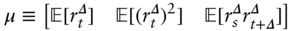
and

Here, refers to the th element in . Next, I estimate by replacing the population moments in (11.5) with their sample counterparts:

where

I calculate autocorrelations to 261 lags, allowing us to test if the returns on a particular date can tell us something about the returns on the same date in the following year. There are too many results to present in full here, but they are well summarized by Figure 11.1.

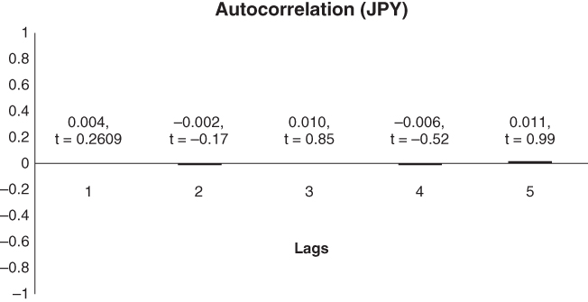
FIGURE 11.1 Autocorrelations in daily JPY data to 5 lags and the corresponding t‐statistics. The t‐statistic is defined as the ratio of the sample autocorrelation and the standard error of the estimate. This number should exceed 1.96 for the calculated autocorrelation to be statistically significant to the 5% level. We are unable to find evidence for statistically significant autocorrelation in any of the currency pairs used in the analysis. The t‐statistics shown above are calculated using a GMM method. The results using the bootstrap method are very similar.

I have not been able to find statistically significant autocorrelations in the data. This holds true across all the currencies in question. Only approximately 5% of the 1566 calculated autocorrelations were statistically significant, corresponding well to the 5% significance level used in the analysis. Our answer to the question posed in this chapter is therefore simply that we cannot find evidence that past returns can be used to predict future returns. This answer holds regardless of whether the GMM or bootstrap method is used to calculate the standard errors. These findings lend support to the martingale assumption used to price FX options.