This chapter tries to cover all the main steps to process and massage data using PySpark. Although the data size we consider in this section is relatively small, but steps to process large datasets using PySpark remains exactly the same. Data processing is a critical step required to perform Machine Learning as we need to clean, filter, merge, and transform our data to bring it to the desired form so that we are able to train Machine Learning models. We will make use of multiple PySpark functions to perform data processing.
Load and Read Data
Assuming the fact that we have Spark version 2.3 installed, we start with importing and creating the
SparkSession object
first in order to use Spark.
[In]: from pyspark.sql import SparkSession
[In]: spark=SparkSession.builder.appName('data_processing').getOrCreate()
[In]: df=spark.read.csv('sample_data.csv',inferSchema=True,header=True)
We need to ensure that the data file is in the same folder where we have opened PySpark, or we can specify the path of the folder where the data resides along with the data file name. We can read multiple datafile formats with PySpark. We just need to update the read format argument in accordance with the file format (csv, JSON, parquet, table, text). For a tab-separated file, we need to pass an additional argument while reading the file to specify the separator (sep='\t'). Setting the argument inferSchema to true indicates that Spark in the background will infer the datatypes of the values in the dataset on its own.
The above command creates a spark dataframe with the values from our sample data file. We can consider this an Excel spreadsheet in tabular format with columns and headers. We can now perform multiple operations on this
Spark dataframe.
[In]: df.columns
[Out]: ['ratings', 'age', 'experience', 'family', 'mobile']
We can print the columns name lists that are present in the dataframe using the “columns” method. As we can see, we have five columns in our dataframe. To validate the number of columns, we can simply use the
length function of
Python.
[In]: len(df.columns)
[Out]: 5
We can use the
count method
to get the total number of records in the dataframe:
We have a total of 33 records in our dataframe. It is always a good practice to print the shape of the dataframe before proceeding with preprocessing as it gives an indication of the total number of rows and columns. There isn’t any direct function available in Spark to check the shape of data; instead we need to combine the count and length of columns to print the shape.
[In]: print((df.count),(len(df.columns))
[Out]: ( 33,5)
Another way of viewing the columns in the dataframe is the
printSchema method
of spark. It shows the datatypes of the columns along with the column names.
[In]:df.printSchema()
[Out]: root
|-- ratings: integer (nullable = true)
|-- age: integer (nullable = true)
|-- experience: double (nullable = true)
|-- family: double (nullable = true)
|-- Mobile: string (nullable = true)
The nullable property
indicates if the corresponding column can assume null values (true) or not (false). We can also change the datatype of the columns as per the requirement.
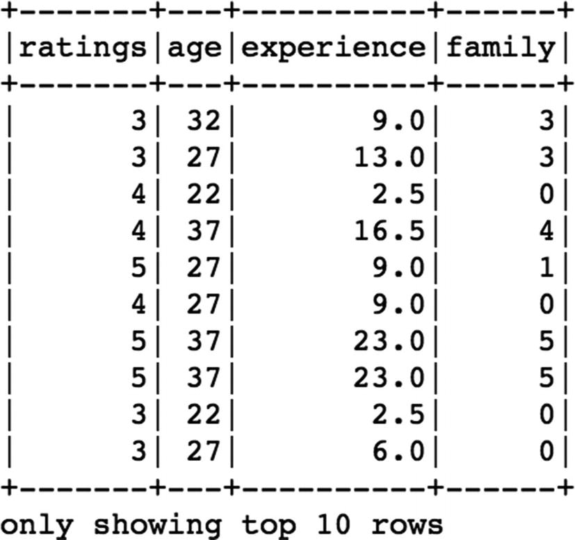
The next step is to have a sneak peek into the dataframe to view the content. We can use the Spark
show method to view the top rows of the dataframe.
We can see only see five records and all of the five columns since we passed the value 5 in the
show method. In order to view only certain columns, we have to use the
select method
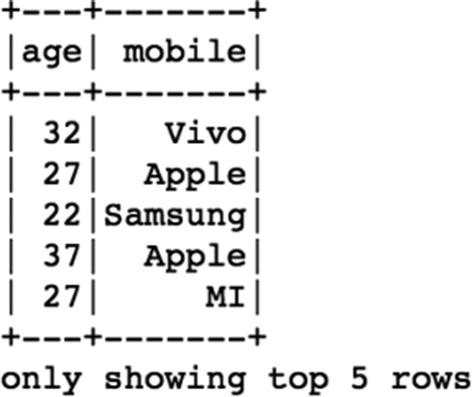
. Let us view only two columns (age and mobile):
[In]: df.select('age','mobile').show(5)
[Out]:
Select function returned only two columns and five records from the dataframe. We will keep using the
select function
further in this chapter. The next function to be used is
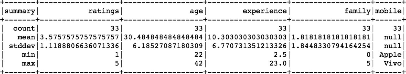
describe for analyzing the dataframe. It returns the statistical measures for each column of the dataframe. We will again use show along with describe, since describe returns the results as another dataframe.
[In]: df.describe().show()
[Out]:
For numerical columns, it returns the measure of the center and spread along with the count. For nonnumerical columns, it shows the count and the min and max values, which are based on alphabetic order of those fields and doesn’t signify any real meaning.
Adding a New Column
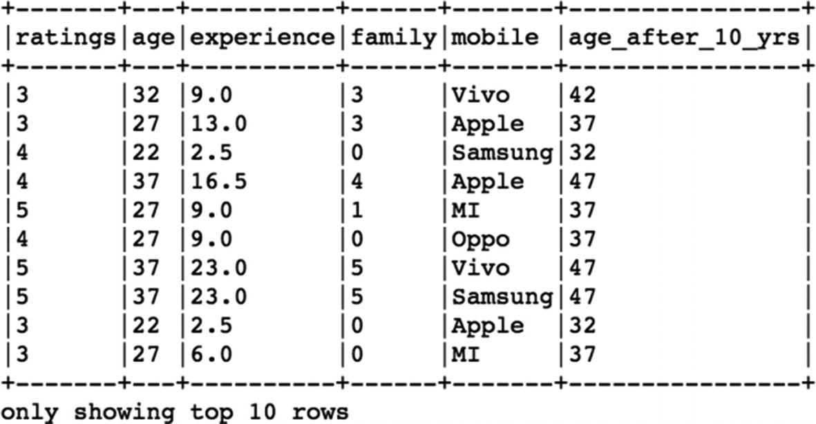
We can add a new column in the dataframe using the
withColumn function of spark. Let us add a new column (age after 10 years) to our dataframe by using the
age column. We simply add 10 years to each value in the
age column.
[In]: df.withColumn("age_after_10_yrs",(df["age"]+10)).show(10,False)
[Out]:
As we can observe, we have a new column in the dataframe. The
show function helps us to view the new column values, but in order to add the new column to the dataframe, we will need to assign this to an exisiting or new dataframe.
[In]: df= df.withColumn("age_after_10_yrs",(df["age"]+10))
This line of code ensures that the changes takes place and the dataframe now contains the new column (age after 10 yrs).
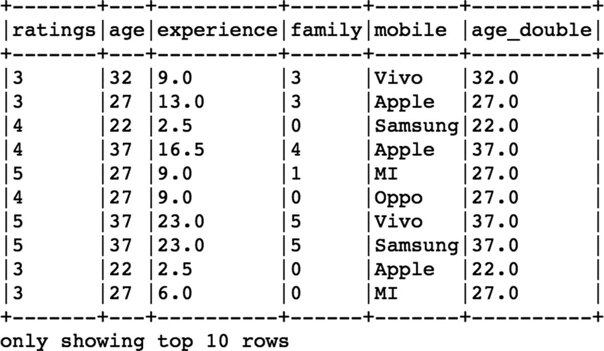
To change the datatype of the
age column from integer to double, we can make use of the
cast method in Spark. We need to import the
DoubleType from
pyspark.types:[In]: from pyspark.sql.types import StringType,DoubleType
[In]: df.withColumn('age_double',df['age'].cast(DoubleType())).show(10,False)
[Out]:
So the above command creates a new column (age_double) that has converted values of age from integer to double type.
Filtering Data
Filtering records based on conditions is a common requirement when dealing with data. This helps in cleaning the data and keeping only relevant records. Filtering in PySpark is pretty straight-forward and can be done using the filter function.
Condition 1
This is the most basic type of filtering based on only
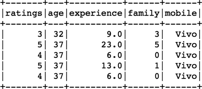
one column of a dataframe. Let us say we want to fetch the records for only ‘Vivo’ mobile:
[In]: df.filter(df['mobile']=='Vivo').show()
[Out]:
We have all records for which
Mobile column has ‘Vivo’ values. We can further select only a few columns after filtering the records. For example, if we want to view the age and ratings for people who use ‘Vivo’ mobile, we can do that by using the
select function after filtering records.
[In]: df.filter(df['mobile']=='Vivo').select('age','ratings','mobile').show()
[Out]:
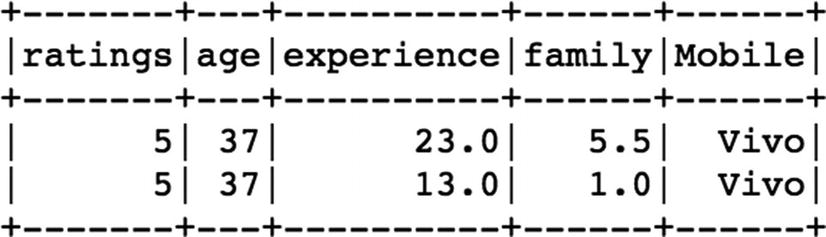
Condition 2
This involves
multiple columns-based filtering and returns records only if all conditions are met. This can be done in multiple ways. Let us say, we want to filter only ‘Vivo’ users and only those with experience of more than 10 years.
[In]: df.filter(df['mobile']=='Vivo').filter(df['experience'] >10).show()
[Out]:
We use more than one filter function in order to apply those conditions on individual
columns. There is another approach to achieve the same results as mentioned below.
[In]: df.filter((df['mobile']=='Vivo')&(df['experience'] >10)).show()
[Out]:
Distinct Values in Column
If we want to view the
distinct values for any dataframe column, we can use the
distinct method. Let us view the distinct values for the m
obile column in the dataframe.
[In]: df.select('mobile').distinct().show()
[Out]:
For getting the count of distinct values in the column, we can simply use
count along with the
distinct function.
[In]: df.select('mobile').distinct().count()
[Out]: 5
Grouping Data
Grouping
is a very useful way to understand various aspects of the dataset. It helps to group the data based on columns values and extract insights. It can be used with multiple other functions as well. Let us see an example of the
groupBy method using the dataframe.
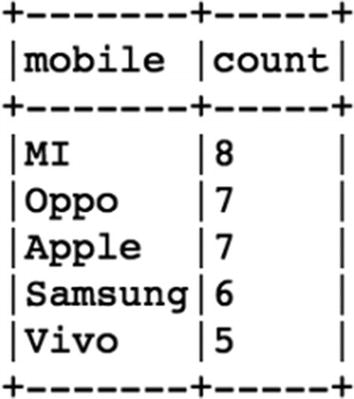
[In]: df.groupBy('mobile').count().show(5,False)
[Out]:
Here, we are grouping all the records based on the categorical values in the m
obile column and counting the number of records for each category using the
count method. We can further refine these results by making use of the
orderBy method to sort them in a defined order.
[In]: df.groupBy('mobile').count().orderBy('count',ascending=False).show(5,False)
[Out]:
Now, the count of the mobiles are sorted in descending order based on each category.
We can also apply the
groupBy method to calculate statistical measures such as mean value, sum, min, or max value for each
category. So let's see what is the mean value of the rest of the columns.
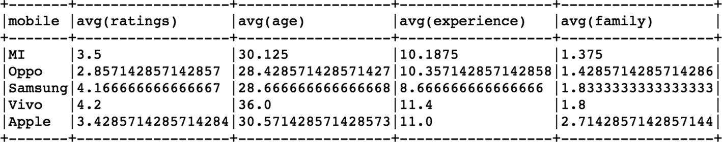
[In]: df.groupBy('mobile').mean().show(5,False)
[Out]:
The
mean method gives us the average of age, ratings, experience, and family size columns for each mobile brand. We can get the aggregated sum as well for each mobile brand by using the
sum method along with
groupBy.
[In]: df.groupBy('mobile').sum().show(5,False)
[Out]:
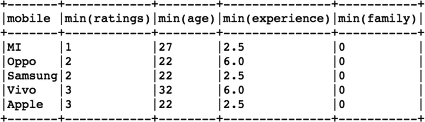
Let us now view the min and max values of users data for every mobile brand.
[In]: df.groupBy('mobile').max().show(5,False)
[Out]:
[In]:df.groupBy('mobile').min().show(5,False)
[Out]:
Aggregations
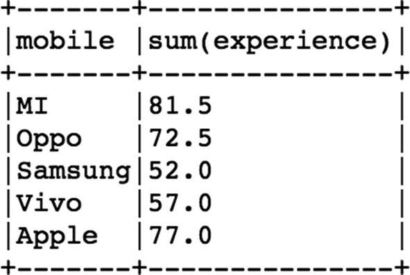
We can use the
agg function
as well to achieve the similar kinds of results as above. Let’s use the
agg function in PySpark for simply taking the sum of total experience for each mobile brand.
[In]: df.groupBy('mobile').agg({'experience':'sum'}).show(5,False)
[Out]:
So here we simply use the agg function and pass the column name (experience) for which we want the aggregation to be done.
User-Defined Functions (UDFs)
UDFs are widely used in data processing to apply certain transformations to the dataframe. There are two types of UDFs available in PySpark: Conventional UDF and Pandas UDF. Pandas UDF are much more powerful in terms of speed and processing time. We will see how to use both types of UDFs in PySpark. First, we have to import
udf from PySpark functions.
[In]: from pyspark.sql.functions import udf
Now we can apply basic UDF either by using a lambda or typical Python function.
Traditional Python Function
We create a simple
Python function, which returns the category of price range based on the mobile brand:
[In]:
def price_range(brand):
if brand in ['Samsung','Apple']:
return 'High Price'
elif brand =='MI':
return 'Mid Price'
else:
return 'Low Price'
In the next step, we create a UDF (
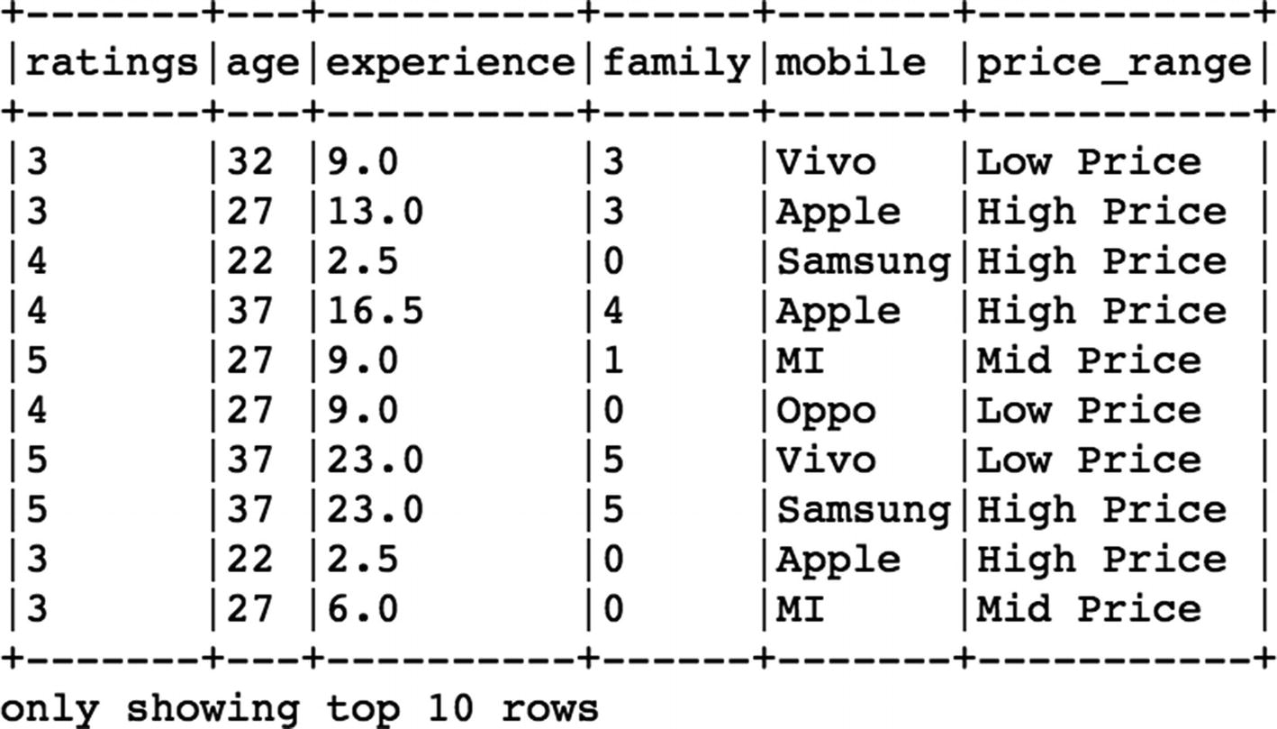
brand_udf) that uses this function and also captures its datatype to apply this tranformation on the mobile column of the dataframe.
[In]: brand_udf=udf(price_range,StringType())
In the final step, we apply the
udf(brand_udf) to the m
obile column
of dataframe and create a new colum (
price_range) with new values.
[In]: df.withColumn('price_range',brand_udf(df['mobile'])).show(10,False)
[Out]:
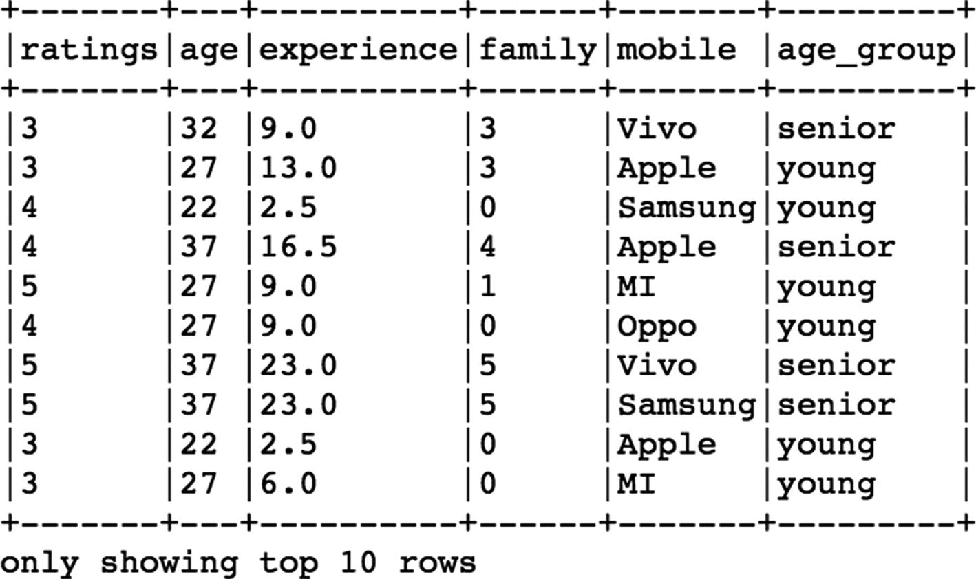
Using Lambda Function
Instead of defining a traditional Python function, we can make use of the
lambda function and create a UDF in a single line of code as shown below. We categorize the age columns into two groups (
young,
senior) based on the age of the user.
[In]: age_udf = udf(lambda age: "young" if age <= 30 else "senior", StringType())
[In]: df.withColumn("age_group", age_udf(df.age)).show(10,False)
[Out]:
Pandas UDF (Vectorized UDF)
Like mentioned earlier, Pandas
UDFs are way faster and efficient compared to their peers. There are two types of Pandas UDFs:
Using Pandas UDF is quite similar to using the basic UDfs. We have to first import
pandas_udf from PySpark functions and apply it on any particular column to be tranformed.
[In]: from pyspark.sql.functions import pandas_udf
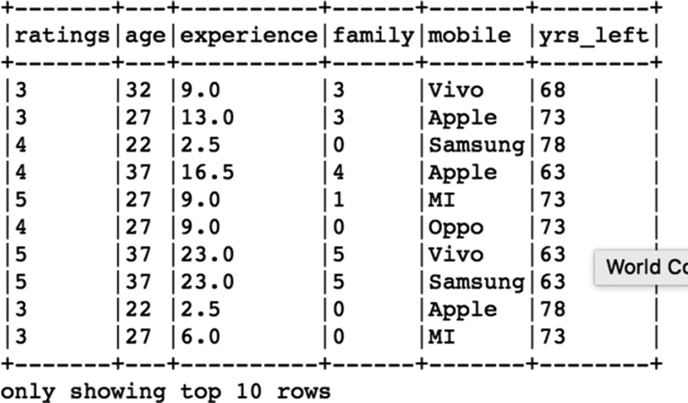
In this example, we define a Python function that calculates the number of years left in a user’s life assuming a life expectancy of 100 years. It is a very simple calculation: we subtract the age of the user from 100 using a Python function.
[In]:
def remaining_yrs(age):
yrs_left=(100-age)
return yrs_left
[In]: length_udf = pandas_udf(remaining_yrs, IntegerType())
Once we create the Pandas UDF (length
_udf) using the Python function (remaining_yrs), we can apply it to the
age column and create a new column yrs_left.
[In]:df.withColumn("yrs_left", length_udf(df['age'])).show(10,False)
[Out]:
Pandas UDF (Multiple Columns)
We might face a situation where we need multiple columns as input to create a new column. Hence, the below example showcases the method of applying a Pandas UDF on multiple
columns of a dataframe. Here we will create a new column that is simply the product of the ratings and experience columns. As usual, we define a Python function and calculate the product of the two columns.
[In]:
def prod(rating,exp):
x=rating*exp
return x
[In]: prod_udf = pandas_udf(prod, DoubleType())
After creating the Pandas UDF, we can apply it on both of the columns (
ratings,
experience) to form the new column (
product).
[In]:df.withColumn("product",prod_udf(df['ratings'],df['experience'])).show(10,False)
[Out]:
Drop Duplicate Values
We can use the
dropDuplicates method
in order to remove the duplicate records from the dataframe. The total number of records in this dataframe are 33, but it also contains 7 duplicate records, which can easily be confirmed by droping those duplicate records as we are left with only 26 rows.
[In]: df.count()
[Out]: 33
[In]: df=df.dropDuplicates()
[In]: df.count()
[Out]: 26
Delete Column
We can make use of the
drop function to remove any of the columns from the dataframe. If we want to remove the m
obile column from the dataframe, we can pass it as an argument inside the
drop function.
[In]: df_new=df.drop('mobile')
[In]: df_new.show()
[Out]:
Writing Data
Once we have the processing steps completed, we can write the clean dataframe to the desired location (local/cloud) in the required format.
CSV
If we want to save it back in the original csv
format as single file, we can use the
coalesce function in spark.
[In]: pwd
[Out]: ' /home/jovyan/work '
[In]: write_uri= ' /home/jovyan/work/df_csv '
[In]: df.coalesce(1).write.format("csv").option("header","true").save(write_uri)
Parquet
If the dataset is huge and involves a lot of columns, we can choose to compress it and convert it into a parquet file format. It reduces the overall size of the data and optimizes the performance while processing data because it works on subsets of required columns instead of the entire data. We can convert and save the dataframe into the parquet format easily by mentioning the format as
parquet
as shown below”.
[In]: parquet_uri='/home/jovyan/work/df_parquet'
[In]: df.write.format('parquet').save(parquet_uri)
Conclusion
In this chapter, we got familiar with a few of the functions and techniques to handle and tranform the data using PySpark. There are many more methods that can be explored further to preprocess the data using PySpark, but the fundamental steps to clean and prepare the data for Machine Learning have been covered in this chapter.