Chapter 4

Deep Learning and Its Parallelization

X. Li; G. Zhang; K. Li; W. Zheng

Abstract

In recent years, deep learning has been extensively studied as a new way to train multilayer neural networks. Deep learning is a set of algorithms in machine learning, which attempts to model high-level abstractions in input data by using multiple nonlinear transformations. Many great achievements of deep learning have been made in speech recognition, computer vision, and natural language processing. Considering that data volume increases rapidly, deep learning becomes more and more important in predictive analytics of big data. We need tens of millions of parameters and billions of samples to train a high quality and practical deep learning model. As the number of parameters and training data are still growing rapidly in the Big Data era, the speed to train a practical model is limited by sequential algorithms and intensive data computation. Therefore, deep learning has been accelerated in parallel with GPUs and clusters in recent years. This chapter introduces several mainstream deep learning approaches developed over the past decades, as well as optimization methods for deep learning in parallel.

Keywords

Big Data analytics; CUDA; Deep learning; GPU; Machine learning; Parallel computing

4.1 Introduction

Big Data has become more and more important because many institutes and companies need to collect useful information from massive amounts of data. Traditional machine learning algorithms were designed to make machines cognize and understand the real world, which means that computers can learn a new knowledge and experience by themselves in a limited dataset with some special customized methods of machine learning. However, it is difficult to learn and analyze in Big Data environment for traditional machine learning algorithms because Big Data has amount of data samples, complicated structures and wide range of varieties. Fortunately, deep learning is a very promising method for solving analytic problems in Big Data. A significant feature of deep learning, which is also the core of Big Data analytics, is to learn high-level representations and complicated structures automatically from massive amounts of raw input data to obtain meaningful information. At the same time, Big Data can provide a large amount of training datasets for deep learning networks, which can help in extracting more meaningful patterns and improve the state of the art performance. Training on large-scale deep learning networks with billions or even more of parameters can dramatically improve the accuracy of the deep networks. But training on those large deep networks involves a large number of forward and backward propagations, which is time-consuming and needs massive amount of computing resources. Therefore, it is necessary to accelerate those large deep networks in high performance computing resources (eg, GPUs, super computers, and distributed clusters).

4.1.1 Application Background

Deep learning is able to find out complicated structures in high-dimensional data, which eventually reaps benefits in many areas of society.

In visual field, the records of image classification have been broken in the ImageNet Challenge 2012 by using deep convolutional neural network (CNN) [1]. Additionally, deep learning has a significant impact on other visual problems, such as face detection, image segmentation, general object detection, and optical character recognition.

Deep learning can also be used for speech recognition, natural language understanding, and many other domains, such as recommendation systems, web content filtering, disease prediction, drug discovery, and genomics [2]. With the improvement of the deep network architectures, training samples and high performance computing, deep learning will be applied successfully in more applications in the near future.

4.1.2 Performance Demands for Deep Learning

Deep learning networks are good at discovering the intricate structures of a multidimensional training data set and are well suited to tackle large-scale learning problems, such as image, audio, and speech recognition. Training on large dataset and large-scale deep networks, which has more layers and huge number of parameters, can result in the state of the art performances. But it also means that training on those large models becomes much more time consuming and we have to wait for a very long time (several months or even years) to get a model well trained. With the rapid development of modern computing device and parallel techniques, it’s possible to train these large-scale models with high performance computing techniques, such as distributed systems with thousands of Central Processing Unit (CPU) cores, Graphic Processing Units (GPUs) with thousands of computing threads and other parallel computing devices.

4.1.3 Existing Parallel Frameworks of Deep Learning

Many research institutes and companies have explored the ability of accelerating deep learning models in parallel. Dean et al. presented that training large deep learning models with billions of parameters using 16,000 CPU cores can dramatically improve training performance [3]. Krizhevsky et al. [1] showed that training a large deep convolutional network with 60 million parameters and 650,000 neurons on 1.2 million high-resolution images can obtain a great performance based on GPU processors. From then on, a lot of frameworks, which are aimed to facilitate researchers experimenting on deep networks, were constantly emerging, including Theano [5], Torch [6], cuda-convnet and cuda-convnet2 [31], Decaf [10], Overfeat [8], and Caffe [7]. Most of these frameworks are open source and optimized by NVIDIA GPUs using Compute Unified Device Architecture (CUDA) programming interface. Moreover, some GPU-based libraries were developed to enhance many of those frameworks, such as the NVIDIA CUDA Deep Neural Network library (cuDNN) [9] and Facebook FFT (fbfft) [11].

The rest of this chapter is organized as follows. In Section 4.2, we will introduce concepts of deep learning, including two fundamental deep learning models, as well as a popular one. In Section 4.3, we will present three popular frameworks of parallel deep learning based on GPU and distributed systems. In the last section, we will discuss challenges and future directions.

4.2 Concepts and Categories of Deep Learning

In this section, we will introduce the concepts of deep learning, including neural networks. And then we will introduce several foundational and popular deep learning models.

4.2.1 Deep Learning

Artificial neural networks

The basic theory of deep learning is from the artificial neural network (ANN) that was a quite popular method of machine learning in the 1980s and 1990s. The idea behind ANN was to develop a novel way for machines to explain and understand data, such as image, speech, and text [4]. The ANN, inspired by the natural neurons, is composed of massive amounts of interconnected computational elements called neurons with numeric weights that can be tuned and be adaptive to inputs.

A simple neural network is shown in Fig. 1. There are four input units and one output. Each input unit (x₁, x₂, x₃, and bias + 1) is multiplied by a weight value W_i and then summed (Eq. 1). The summed value will be taken as the input of the activation function: f(z).

hw,bx=fWTx=f∑i=13Wixi+b

  (1)

Fig. 1 A simple neuron network.

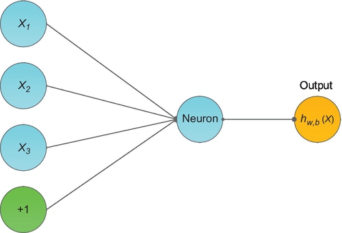
We can choose sigmoid function (one of the activation functions that commonly used in deep learning models) to act as activation function (Eq. 2):

fz=11+e−z

  (2)

The single neuron was explained exactly according to the mapping relationship between input and output by logistic regression [5].

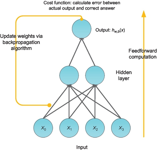
A neural network consists of many simple neurons and more layers (Fig. 2).

Fig. 2 Neuron network with three layers.

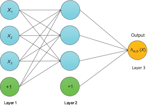
As shown in Fig. 2, the neural network is composed of three layers, four inputs, and one output. The leftmost layer is input layer that consists of three inputs (x₁, x₂, x₃) and one bias unit. The rightmost layer is called an output layer with a single output unit. In the middle of the network, layer L2 is called the hidden layer.

One can extend the neural network by adding input and a hidden layer to train a large problem. Researchers have created many kinds of ANN models and those models have been applied in the field of artificial intelligence, such as pattern recognition, time series prediction, signal processing, control, soft sensors, anomaly detection, and so on. However, when learning from more complicated problems, ANN mainly has several restrictions [6]:

• It requires a huge amount of training data to train the network for a decent model.

• A neural network is prone to overfitting.

• The parameter of a neural network is difficult to be tuned.

• A neural network has limited ability to identify complicated relationships.

• The configuration of a neural network is empirical and many methodologies have not yet been figured out.

• A neural network is time consuming.

Because of the above restrictions, ANN was not applied extensively. Deep learning has the same network structure as ANN’s, but deep learning has totally different training methods.

Concept of deep learning

The idea of deep learning was based on ANNs, but deep learning methods can automatically extract a complex data representation and identify more complicated relationships between input and output.

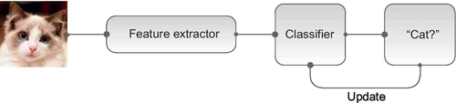
In a conventional machine learning model, the engineer and researcher were required to design a feature extractor manually from raw input data before classifying an object (Fig. 3). In comparison to a deep learning model, the key limitation of machine learning is that it cannot efficiently generate complicated and nonlinear patterns automatically from raw input data.

Fig. 3 Classification process in traditional machine learning.

From 2006, a new research area of machine learning named deep structured learning or deep learning was introduced to the world. In comparison to conventional machine learning, the engineer and researcher do not need to extract features manually. Instead, these features can be generated automatically by using deep learning. We can refer to the following definition of deep learning: “Deep learning is a new area of machine learning research, which has been introduced with the objective of moving machine learning closer to one of its original goals: artificial intelligence. Deep learning is about learning multiple levels of representation and abstraction that help to make sense of data such as images, sound, and text” [13].

In recent years, compared to deep structured model, research in machine learning and signal process has explored shallow structured models that usually contain one or two layers of nonlinear feature transformations, such as Gaussian mixture models, support vector machines, extreme learning machines, and so on. Many shallow models are a good choice to solve simple or well-constrained problems, but they are inefficient in handling more complicated applications such image recognition, speech recognition, and natural languages understanding.

The mainstream models in deep learning are mainly divided into three classes: supervised learning, unsupervised learning, and hybrid learning model. The model of unsupervised learning can be used to cluster the input based on their statistic properties without being provided with the correct answer during the training. Main unsupervised learning models include:

• Auto-encoders

• Stacked denoising auto-encoders

• Restricted Boltzmann machines

• Deep belief networks

In contrast, the training dataset of a supervised learning model includes both the input data and the desired output (correct answer) data during the training process. Supervised learning models include:

• Logistic regression

• Multilayer perceptron

• Backpropagation (BP)

• Deep convolutional network

In addition, practitioners usually complement hybrid models that are combined with the use of unsupervised model and supervised model. In the hybrid models, in order to initialize the preset training parameters to sensible values, unsupervised learning is used as a pretraining method and extracts more useful features for the supervised model.

4.2.2 Mainstream Deep Learning Models

Autoencoders

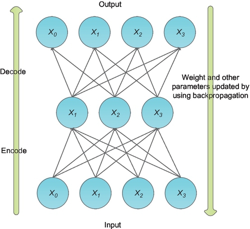
An autoencoder was first designed in the 1980s by Hinton to address unsupervised learning problems. It has two or three layers of a neural network and applies BP to learn nonlinear codes to reconstruct the input data. It aims at learning an identity equation, which makes the output approximately equal to input (Eq. 3). In fact, some interesting structures of the input data can be found by making some constraints on the hidden layer of the network (like limiting the number of hidden units) [12]. If given a set of unlabeled training dataset (x₀, x₁, x₂, …), x_i is N dimensional. Fig. 3 shows how autoencoder model works:

hxi;w,b=xi

  (3)

minimizew,b∑i=0m∥hxi;w,b−xi∥

  (4)

There are three layers in an autoencoder model (Fig. 4): input layer, hidden layer, and output layer. The hidden layer is forced to compress the input data into a high-level representation, which is called “encode the input data.” After encoding, the network minimizes the objective function by BP that adjusts weight values and other parameters according to output (Eq. 4).

Fig. 4 A simple model of the autoencoder.

Backpropagation

BP was introduced in the 1970s and has become the workhorse of learning in neural networks. You can see a simple three-layer BP network model in Fig. 5.

Fig. 5 A simple model of the backpropagation algorithm.

BP algorithm mainly consists of two computing processes: feedforward and back propagation. When in feedforward pass, the BP model computes the outputs to each hidden layer and then squashes the outputs using activation functions (such as sigmoid function). It then repeats the process with the output layer. If the actual output (h_w,b(x)) is different with the expected output (label (y)), the back propagation begins. In a BP pass, the model will apply the BP equation repeatedly to propagate gradients through all the layers, from the output layer all the way to the input layer [2]. During BP, the weights of each layer will be updated according to these gradients in order to minimize the cost function: J(w, b; x, y) (Eq. 5). Given a set of training samples:

x1,y1,x2,y2,…xm,ym

For a single training sample: (xⁱ, yⁱ), we can define the cost function as follows (Eq. 5):

Jw,b;x,y=12∥hw,bx−y2∥

  (5)

When the difference between the actual output and expected output has become small enough, or the network reaches a preset number of stop iterations (Epoch_max), the algorithm will stop the training. You can see the detailed mathematical equation and derivation in [14–16]. The whole BP algorithm flow shows in Fig. 6. The summary of the BP algorithm is as follows:

Fig. 6 BP training flowchart.

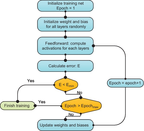
Step 1: Initialize the training net: Construct a new BP network and its parameters, set some necessary parameters (eg, the learning rate), and randomly initialize the weights and bias to small values between − 1 and + 1.

Step 2: Randomly choose an input from training samples and conduct the feed-forward computation.

Step 3: Calculate the errors (E) between the actual output and expected output.

Step 4: Check against the stopping criteria.

Step 5: If it does not meet the stop condition, it conduct the back propagation (computes the gradients and update weights). After Step 5 is finished, return to Step 2.

Convolutional neural network

The most popular deep learning models used to train image data are known as convolutional neural networks (CNNs). The inspiration of CNNs is from Hubel and Wiesel’s early research on cat’s visual cortex [16]. It was designed to handle multiple array problems, such as signal and sequences, images, speech, videos, etc. [2]. CNNs have achieved great success in image recognition, speech recognition, and natural language understanding.

Architecture overview of CNNs

Essentially, deep CNNs are typical feedforward neural networks, which are applied BP algorithms to adjust the parameters (weights and biases) of the network to reduce the value of the cost function. However, it is very different from the traditional BP networks in four new conceptions: local receptive fields, shared weights, pooling, and combination of different layers. A typical structure of CNNs is shown in Fig. 7 (LeNet-5) [21].

Fig. 7 The simple architecture of CNN (LeNet-5).

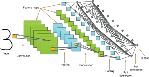
The network consists of one or more convolutional layers (often followed by a subsampling layer), and then ends with one or more fully connected layers.

Input layer

The input layer can be images, sounds, or one or more real numbers. In the example of LeNet-5, the input data is two-dimensional (2D) arrays of pixels. Generally, each input image will be an M × N × K real array. M and N are the height and width of the image and K is the number of channels per pixel (eg, an RGB image has K = 3). For example, the input image is a 28 × 28 × 3 real array in LeNet-5.

Convolutional layer

After the input layer received the input images, these images will be convolved by the convolution layer, which consists of a set of different learnable filter banks of size m × n × r. Each filter is smaller than the input size, but it extends through the full depth of the input volume. During the convolution, each filter bank will be slid across the height and width of the input images, generating a 2D feature map of that filter. When we slide the filter across the input image, we compute the dot production between the values of the filter and the input and then pass the result of the dot production into a non-linearity activation function (such as a ReLU, Sigmoid, and Tanh). For each filter bank, we repeat the above convolution operations and then a set of 2D feature maps will be generated as the output of convolutional layers. The number feature maps are the same as the number filter banks, and all neurons in the same feature map share the same weights (filter bank).

Local connectivity. Unlike the traditional fully connected neural networks, each neuron of the feature map in CNNs is only connected to a local region of the input. This spatial extent of connectivity is named a local receptive field. With these local receptive fields, elementary features like oriented edges, endpoints, and corners can be extracted and then combined to detect higher-level features by the subsequent layers.

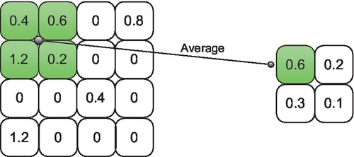
Pooling layer

After each convolutional layer, it is commonly to insert a pooling layer. Pooling layers can reduce the resolution of feature maps, and thus reduce the amount of parameters and computation in CNNs. Pooling layers are also can be used to control the over-fitting problems [19]. There are two methods of pooling: max pooling and average pooling, and that means each pooling unit calculates the maximum or average of a local patch in one feature map. A simple example of average pooling is shown in Fig. 8.

Fig. 8 Example of average pooling.

Full connection layer

The full connection layer is the same as the traditional neural networks, in which neurons have full connections to all activations with the previous layer.

4.3 Parallel Optimization for Deep Learning

It has been found that the accuracy of deep learning models will be greatly improved by increasing the scale and the number of parameters in the deep model. But it also means we have to spend more time to train these large-scale deep learning models. The traditional serial algorithms are hard to handle these large deep models in a fast speed. Therefore, parallelizing the deep learning model is necessary. The parallel of deep learning has been explored for many years and the main development is shown in Table 1.

Table 1

The Development of Deep Learning Model in Parallel

Solution	Contribution
CPU to multicore CPUs	Train the model in parallel by using different cores
Multicore CPUs to GPU	Train the model in parallel by GPU by using huge numbers of threads in a GPU device with zero schedule overhead and powerful float computing ability
GPU to multi-CPUs	Train large-scale deep neural network by using CPU clusters for the sake of the limitation of single GPU memory
Multi-CPUs to multi-GPUs	The problem of limited memory of a single GPU does not exist when using multi-GPUs to train the large-scale deep networks

In this section, we will introduce two popular parallel frameworks and discuss a general parallel method of the large deep learning model.

4.3.1 Convolutional Architecture for Fast Feature Embedding

Convolutional architecture for fast feature embedding (Caffe) was aimed to provide a clean, quick start and a modular deep learning framework for scientists in research area and industry. It was developed and maintained by Berkeley Vision and Learning Center (BVLC) and community contributors.

Caffe is one of the most popular deep learning frameworks due to five good points: expressive architecture, extensible code, fast training speed, open source, and active community. The users don’t have to rewrite the code of Caffe to set up new deep neural networks. Instead, they just need to modify several lines of configuration files to start a new network. Computation mode between CPU and GPU can be easily switched by changing a single line flag [20].

CUDA programming

GPU is extensively used as a computational device, thanks to its excellent computational power and parallel hardware architecture with thousands of arithmetic logic unit (ALU) cores. We can see the difference in computational power between GPUs and CPUs in Fig. 9.

Fig. 9 Performance between CPU and GPU.

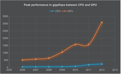
The large gap of the performance lies in the different design philosophy between GPUs and CPUs. The design of CPU is that more transistors on the chip are used for control and cache units, while most of the transistors on GPU are used for computational units and few for control and cache, which makes GPU handle multiple tasks more efficiently [18].

The architecture of GPU

GPU is connected to the host device through the PCI Express (PCIe) and it has its own device memory that is up to several gigabytes in modern devices. GPU hardware mainly consists of memory, streaming multiprocessors (SMs), and streaming processors (SPs).

GPU is an array of SMs that consist of SPs and memory (Fig. 10). Each SM can execute in parallel with the others. NVIDIA Kepler k40 has 15 multiprocessors and 2880 cores and each core can execute a sequential thread in SIMT (single instruction, multiple thread). Each SM is associated with a private shared memory (L1 cache), read-only texture memory, registers, L2 cache, etc. Each core has a fully pipelined integer ALU, a floating point unit, a move and compare unit, and a branch unit [17,18].

Fig. 10 A simplified architecture of GPU hardware.

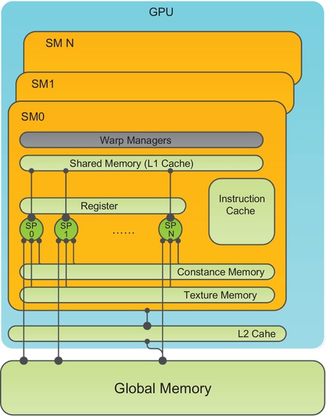
Each thread can access register and shared memory at a very high speed in parallel, and we also refer to shared memory as on-chip memory. Registers are private to individual threads, and each thread can only access its own registers. Thirty-two threads are grouped into a warp, which is scheduled by a warp manager, and the threads in a warp are executed in SIMT mode. The computational ability can be enhanced by extending more SMs and memory resources.

CUDA programming framework

In 2007, the CUDA was introduced to the world. This easy-to-use program framework pushed the development of GPGPU and allows the programmer to write codes without having to learn complicated shader languages. CUDA supports high-level programming languages such as C/C++, Fortran, and Python.

A grid consists of many thread blocks and a thread block is a group of threads. Warps are the basic execution unit on SM. When thread blocks are dispatched into a certain SM, the threads in the thread block are grouped into warps (32 consecutive threads) (Fig. 11).

Fig. 11 Thread organization of CUDA.

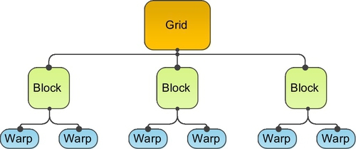
Thread. A thread runs on the individual core of SM and executes an instance of the kernel. Each thread has a thread ID within in its thread block, program counter, register, per-thread private, inputs, and output results.

Block. Each block is a logical unit that contains a number of threads. A block is an array of concurrent threads that cooperate to compute a result. The threads of a block can be indexed by using 1D, 2D, or 3D indexes.

Grid. A grid is an array of blocks that are all running on the same kernel. Each grid reads from global memory, writes results to global memory, and synchronizes between dependent kernel calls.

Warp. The warp is the basic execution element on GPU and CUDA codes actually run as warp. The size of a warp depends on GPU hardware. Each CUDA core executes 32 threads simultaneously on K40c. At runtime, a block is divided into a number of warps.

A GPU can execute one or more kernel grids and an SM can execute one or more thread blocks. If you want to run program on GPU, you should define kernel functions that N different CUDA threads execute in parallel.

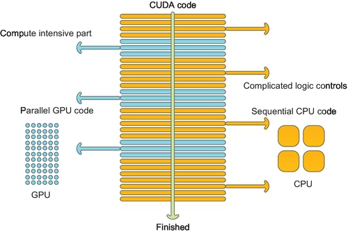
In CUDA program framework, GPU works as a coprocessor of the CPU. The program is switched to GPU when kernel function is called for by the CPU. CPU is optimized for low-latency access to cached data sets and control logic; therefore, it is well suited for those serial codes with complicated logic control. Instead, GPU is optimized for data-parallel and throughput computation, so it is good for the computational intensive work (Fig. 12).

Fig. 12 The execution mode of CUDA code.

Architecture of Caffe

Data storage in Caffe

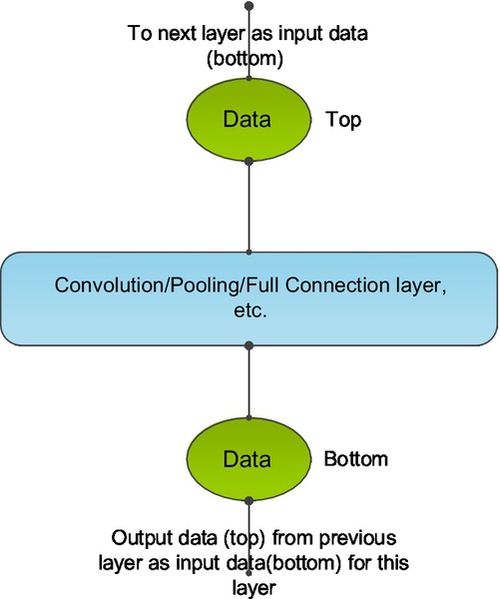
All the data (such as images, weights, biases, and derivatives) in Caffe is stored in a 4D array which is called a blob. For example, the batches of images data in 4D blobs are stored like this: Number × Channel × Height × Width.

For each layer, the input data are stored in the bottom blob and the output data are in the top blob (Fig. 13), while the next layer will take the top blob from the previous layer as its input data (bottom blob).

Fig. 13 Layer communication in Caffe.

Layer topology in Caffe

The essence of different networks is the different combination of functional layers. Caffe supports a complete set of functional layers like convolution, pooling, inner products, nonlinearities, and losses [20].

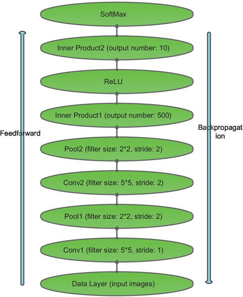
A simple example of LeNet architecture in Caffe is shown in Fig. 14. The operations of these layers are convolution, pooling, full connection, and SoftMax. In the forward phase, the computation of the input data starts from the data layer at the bottom all the way to the output layer at the top. The BP algorithm is applied to compute the gradients in the backward phase and update parameters for each layer.

Fig. 14 A simple example of LeNet topology in Caffe.

Parallel implementation of convolution in Caffe

In all of the deep CNNs, convolution operations are computationally expensive and dominant most of the runtime. Therefore, an important way to improve performance of the whole network is to reduce the runtime of convolution.

There are three approaches to implement convolution operations. The first common way is to compute the convolution directly. This will be efficient when batch sizes are large enough and inefficient when the batch size is below 64 [9]. The second approach is to employ the fast Fourier transform to compute the convolution, which can lower the complexity of the convolutions [11]. This way has turned out to be the fastest convolution, but it is limited by memory consumption. The third way is to unroll the convolution into a large matrix. After unrolling the convolution, the computation of each convolution turns to a matrix-matrix production by using highly efficient libraries (eg, cuBLAS). The NVIDIA CUDA Basic Linear Algebra Subroutines (cuBLAS) is a deeply GPU-optimized version of the BLAS library [22], which is very efficient for matrix-matrix production.

The third convolution approach is used in Caffe: The local regions of the input image are unrolled into columns and the weights of the convolution layer are similarly unrolled into rows. Therefore, the result of a convolution is turned to one large matrix multiply. The unrolling operation in Caffe is in a function called im2col_gpu; then, cuBLAS can be used efficiently for matrix-matrix production. Because there is an overlap of the receptive fields in convolution, most numbers in the input may be duplicated in the unrolled large matrix. The results of matrix production must be reshaped to proper output dimension. The detailed computing flow of convolution in Caffe is shown in Fig. 15.

Fig. 15 Computing the flow of the convolution layer in Caffe.

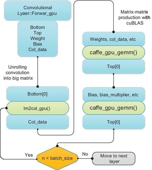
Fixed steps are used in Caffe to train the model, and the program only processes one images of a batch during an iteration. The computing flow as follows:

Step 1: Data preparation, such as input, output, weights, and bias for im2col_gpu. The input data of convolution layer is stored in bottom blob and output in top blob. Before training, the weight and biases need to be initialized randomly.

Step 2: Unroll the convolution data into large matrix. The image is transformed into a big matrix in parallel by using im2col_gpu. The result of unrolling is stored in col_data.

Step 3: The funtion caffe_gpu_gemm is called to conduct matrix multiplication between unrolled input and weights on GPU by using cuBLAS.

Step 4: The function caffe_gpu_gemm is called to conduct matrix multiplication between unrolled input and bias on GPU by using cuBLAS.

Step 5: Check stop criteria. If all images in a batch are processed, the program moves to next layer. Otherwise, go to Step 2.

4.3.2 DistBelief

Introduction of DistBelief

It was reported by the New York Times in 2012 that Google DistBelief [3] could identify the key features of a cat from millions of You Tube videos. The key technique behind DistBelief is deep learning. Moreover, DistBelief is a very complicated and large distributed system composed by 1000 machines, including a total of 16,000 cores and 1 billion network parameters. This parallel deep learning framework supports model parallelism both within a machine by multithreading and across machines by message passing. Meanwhile, it also supports data parallelism to train different replicas of a model. The main algorithms in DistBelief are Downpour stochastic gradient descent (SGD) and L-BFGS. It has been applied in image classification and speech recognition fields [23].

A significant advance has been brought by using GPU to train deep learning networks. But the bottleneck using GPU to train large deep networks with billions of training examples and parameters is the limitation of a single GPU memory. DistBelief was designed to address this problem, and it provides an alternative method to train a large deep network by using large-scale clusters in distributed way [24].

Downpour SGD

Many researchers have accelerated machine learning algorithms by distribution methods before DistBelief [25–27]. SGD is extensively applied in deep learning algorithms to reduce output error. The designer of DistBelief provides us with Downpour SGD, a new method suitable for distributed systems. The key advantages of Downpour SGD are asynchronous stochastic gradient, adaptive learning rates and numerous model replicas. Compared to traditional SGD, the convergence rate of Downpour SGD has been improved significantly.

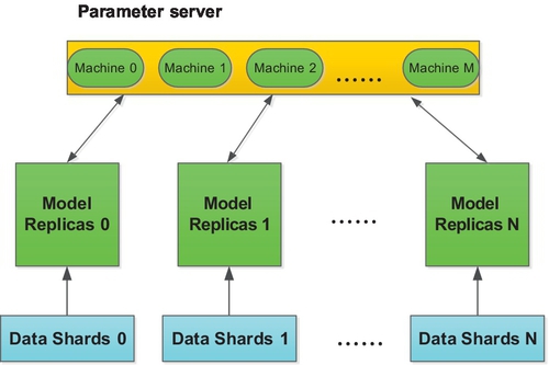
The basic idea of Downpour SGD is as follows: The training samples are divided into different small parts and each model replica computes gradients for each small part. Before each model replica starts to train its small part, the model replica sends a request to parameter server to ask for the latest parameter (Fig. 16). When the model replica receives the latest parameter from parameter server, it begins to compute parameter gradients for its own small part and sends the gradients result back to the parameter server. The parameter server will be updated with the latest gradients. In this way, the parameter can hold the latest state of parameters for the model. The parameter server consists of different machines, and the total workload is averaged by each machine in parameter server [24].

Fig. 16 The basic idea of Downpour SGD.

Sandblaster L-BFGS

Training deep networks on batch can get good performances in small deep networks [26,27], but it is not well suited for large deep networks. The Sandblaster batch optimization framework (L-BFGS) was introduced to address this problem.

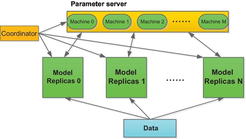
In Sandblaster L-BGGS algorithm, each model replica runs on the whole training sample. The key idea of the algorithm resides in the coordinator (Fig. 17), which sends a set of commands to store and manipulate model parameters distributively [24].

Fig. 17 The basic idea of Sandblaster L-BGGS.

4.3.3 Deep Learning Based on Multi-GPUs

The data in deep learning can be divided into two types of data: parameters and input/output data. Parameters in CNNs include the learning rate, convolutional parameters (eg, filter numbers, kernel size, and stride), pooling parameters (kernel size, stride), bias, etc. Input data includes the raw data (eg, images and speeches) received from the input layer, and output data keep the intermediate output of each layer, such as the convolutional and pooling layers. The key to train large scale CNN models with multiple GPUs is how to divide tasks between different GPUs. We have three ways to train these large models with multiple GPUs: data parallelism, model parallelism, and data-model parallelism.

Data parallelism

Data parallelism can be easily implemented and it is thus the most widely used implementation strategy on multi-GPUs.

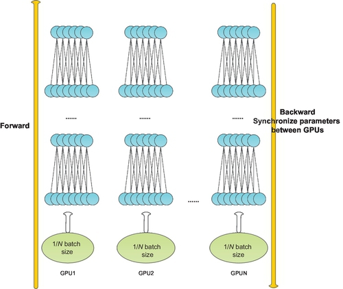
Data parallelism means that each GPU uses the same model to trains on different data subset. In data parallel, there is no synchronization between GPUs in forward computing, because each GPU has a fully copy of the model, including the deep net structure and parameters. But the parameter gradients computed from different GPUs must be synchronized in BP (Fig. 18).

Fig. 18 The illustration of data parallelism mode.

Model parallelism

Model parallelism means that each computational node is responsible for parts of the model by training the same data samples.

The model is divided into several pieces and each computing node such as GPU is responsible for one piece of them (Fig. 19). The communication happens between computational nodes when the input of a neuron is from the output of the other computational node. The performance of model parallelism is often worse than data parallelism, because the communication expenses from model parallelism are much more than that of data parallelism.

Fig. 19 The illustration of model parallelism mode.

Data-model parallelism

Several restrictions exist in both data parallelism and model parallelism. For data parallelism, we have to reduce the learning rate to keep a smooth training process if there are too many computational nodes. For model parallelism, the performance of the network will be dramatically decreased for the sake of communication expense if we have too many nodes.

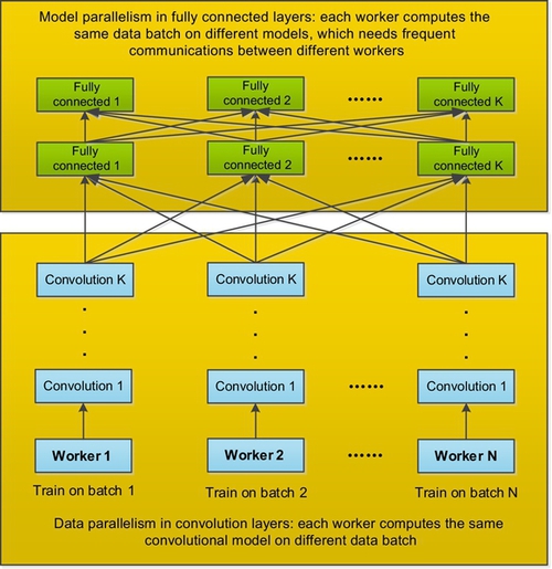
Model parallelism could get a good performance with a large number of neuron activities, and data parallel is efficient with large number of weights. In CNNs, the convolution layer contain about 90% of the computation and 5% of the parameters, while the full connected layer contain 95% of the parameters and 5%-10% the computation. Therefore, we can parallelize the CNNs in data-model mode by using data parallelism for convolutional layer and model parallelism for a fully connected layer (Fig. 20).

Fig. 20 The illustration of data-model parallelism mode.

Example system of multi-GPUs

Facebook designed a parallel framework by using four NVIDIA TITAN GPUs with 6 GB of RAM on a single server in data parallel and model parallel. ImageNet 2012 dataset can be trained in 5 days [28].

Commodity Off-The-Shelf High Performance Computing (COTS HPC) system was designed by Google to train large-scale deep networks on more than 1 billion parameters. COTS HPC consists of GPU servers with Infiniband interconnections, and the communication between different GPUs is controlled by Message Passing Interface (MPI). The training of a large deep net with more than 1 billion parameters was completed in 3 days on COTS HPC [29]. The same experiment was done by DistBelief, but COTS HPC provides us with a much cheaper and faster way of doing it.

4.4 Discussions

4.4.1 Grand Challenges of Deep Learning in Big Data

With the development of powerful computing devices (eg, GPUs), the potentially valuable datasets provided by Big Data and the advanced CNN architecture, deep learning models are promising to fully make use of huge amounts of data to mine and extract meaningful representations for classification and regression. However, deep learning poses some specific challenges in Big Data, including processing massive amounts of training data, learning from incremental streaming data, the scalability of deep model, and learning speed.

Massive amounts of training sample

Generally, learning from a large number of training samples provided by Big Data can obtain complex data representations (features) at high levels of abstraction which can be used to improve the accuracy of classification of the deep model. An obvious challenge of deep learning in Big Data is the various formats of datasets. Including high dimensionality data, massive unsupervised or unlabeled data, noisy and poor quality data, highly distributed input sources imbalanced input data, etc. [30]. The existing deep learning algorithms cannot adapt to train such various kinds of training samples, and thus dealing with data diversity is a really big challenge to current deep learning models.

Incremental streaming data

Streaming data is one of the key features of Big Data, which is large, fast moving, dispersed, unstructured, and unmanageable. Such data extensively exist in many areas of society, including websites, blogs, news, videos, telephone records, data transfer, and fraud detection [30]. One of the big challenges of learning meaningful information with deep learning models from streaming data is how to adapt deep learning methods to handle such incremental and unmanageable streaming data.

Learning speed in Big Data

The big challenge in training speed of deep learning is mainly from two aspects: the large scale of the deep network and the massive amount of training samples provided by Big Data. It has been turned out that a large-scale CNN models that have a complicated architecture (with more than billions of parameters and much more layers) are able to extract more complicated features and thus improve the state of the art performance, and accordingly, the training become prohibitively computationally expensive and time-consuming. Besides, training a deep model on a huge amount of training data is also time-consuming and requires a large amount of compute cycles. Consequently, how to accelerate the training speed of those large-scale models in Big Data environment is a big challenge.

Scalability of deep models

To train large-scale deep learning models faster, an important method is to accelerate the training process with distributed computing and powerful computing devices (eg, clusters and GPUs). The existing approaches of parallel training includes data parallel, model parallel, and data-model parallel. But when training on large-scale deep models, each of them will be of low efficiency for the sake of parameter synchronization that needs frequent communications between different computing nodes (such as different server nodes in distributed system, and heterogeneous computing systems between CPU and GPUs). Additional, the memory limitation of modern GPUs can also lead to scalability of deep networks. The big challenge is how to optimize and balance workload computation and communication in large-scale deep learning networks.

4.4.2 Future Directions

Big data provides us with a very important chance to improve the existing deep learning models and to propose novel algorithms to address specific problems in Big Data. The future work will focus on algorithms, applications, and parallel computing.

In the perspective of algorithms, we have to research how to optimize the existing deep learning algorithms or explore novel approaches of deep learning to train massive amounts of data samples and streaming samples from Big Data. Moreover, we also need to create novel methods to support Big Data analytics, such as data sampling for extracting more complex features from Big Data, incremental deep learning methods for dealing with streaming data, unsupervised algorithms for learning from massive amounts of unlabeled data, semi-supervised learning, and active learning.

Application is one of the most researched areas in deep learning. Many traditional research areas have benefited from deep learning, such as speech recognition, visual object recognition, and object detection, as well as many other domains, such as drug discovery and genomic. The application of deep learning in Big Data also needs to be explored, such as generating complicated patterns from Big Data, semantic indexing, data tagging, fast information retrieval, and simplifying discriminative tasks.

The last important point of future work is parallel computing in deep learning. We could research existing parallel algorithms or open source parallel frameworks and optimize them to speedup training process. We could also propose novel distributed and parallel deep learning computing algorithms and frameworks to support quick training of large-scale deep learning models. However, to train a larger deep model, we have to figure out the scalability problem of large-scale deep models.

References

[1] Krizhevsky A., Sutskever I., Hinton G. ImageNet classification with deep convolutional neural networks. In: Proc. Advances in Neural Information Processing Systems 25; 2012:1090–1098.

[2] LeCun Y., Bengio Y., Hinton G. Review: Deep learning. Nature. 2015;521:436–444.

[3] Dean J., Corrado G., Monga R., Chen K., Devin M., Mao M., et al. Large scale distributed deep networks. Adv Neural Inf Process Syst. 2012;25:1232–1240.

[4] Schmidhuber J. Deep learning in neural networks: an overview. arXiv: 1404.7828, 2014.

[5] http://deeplearning.stanford.edu/wiki/index.php/Neural_Networks.

[6] Tu J.V. Advantages and disadvantages of using artificial neural networks versus logistic regression for predicting medical outcomes. J Clin Epidemiol. 1996;49(11):1225–1231.

[7] Jia Y, Shelhamer E, Donahue J, Karayev S, Long J, Girshick R, et al. Caffe: convolutional architecture for fast feature embedding. arXiv. preprint arXiv:1408.5093, 2014.

[8] Sermanet P., Eigen D., Zhang X., Mathieu M., Fergus R., LeCun Y. Overfeat: integrated recognition, localization and detection using convolutional networks. In: ICLR; 2014.

[9] Chetlur S, Woolley C, Vandermersch P, Cohen J, Tran J, Catanzaro B, et al. cudnn: efficient primitives for deep learning. CoRR, abs/1410.0759, 2014. http://arxiv.org/abs/1410.0759.

[10] Donahue J, Jia Y, Vinyals O, Hoffman J, Zhang N, Tzeng E, et al. Decaf: a deep convolutional activation feature for generic visual recognition. CoRR, abs/1310.1531, 2013.

[11] Vasilache N, Johnson J, Mathieu M, Chintala S, Piantino S, LeCun Y. Fast convolutional nets with fbfft: a GPU performance evaluation. arXiv: 1412.7580, 2015.

[12] http://deeplearning.stanford.edu/wiki/index.php/Autoencoders_and_Sparsity.

[13] https://github.com/lisa-lab/DeepLearningTutorials.

[14] http://deeplearning.stanford.edu/wiki/index.php/Backpropagation_Algorithm.

[15] LeCun Y., Bottou L., Orr G., Muller K. Efficient BackProp. In: Orr G., Muller K., eds. Neural networks: tricks of the trade. Heidelberg: Springer; 1998.

[16] Hubel D., Wiesel T. Receptive fields and functional architecture of monkey striate cortex. J Physiol (London). 1968;195:215–243.

[17] http://www.nvidia.com/object/what-is-gpu-computing.html.

[18] NVIDIA, Tesla K40 GPU Active Accelerator. BD-06949-001_V03, 2013.

[19] He K., Zhang X., Ren S., Sun J. Spatial pyramid pooling in deep convolutional networks for visual recognition. In: ECCV; 2014.

[20] http://caffe.berkeleyvision.org/.

[21] Tompson J, Jain A, LeCun Y, Bregler C. Joint training of a convolutional network and a graphical model for human pose estimation. CoRR, abs/1406.2984, 2014.

[22] https://developer.nvidia.com/cublas.

[23] Zinkevich M., Weimer M., Smola A., Li L. Parallelized stochastic gradient descent. In: NIPS; 2010.

[24] Le Q.V., Ngiam J., Coates A., Lahiri A., Prochnow B., Ng A.Y. On optimization methods for deep learning. In: ICML. 2011.

[25] Agarwal A., Duchi J. Distributed delayed stochastic optimization. In: NIPS; 2011.

[26] Niu F., Retcht B., Re C., Wright S.J. Hogwild. A lock-free approach to parallelizing stochastic gradient descent. In: NIPS; 2011.

[27] Dean J., Corrado G.S., Monga R., Ng A.Y., et al. Large scale distributed deep networks. In: Advances in Neural Information Processing 25 (NIPS 2012). Cambridge, MA: MIT Press; 2012.

[28] Yadan O, Adams K, Taigman Y, Ranzato MA. Multi-GPU training of ConvNets. arXiv: 1312.5853v4 [cs.LG] (February 2014).

[29] Coates A., Huval B., Wang T., Wu D.J., Ng A.Y., Catanzaro B. Deep learning with COTS HPC systems. In: Proc. International Conference on Machine Learning (ICML’13); 2013.

[30] Najafabadi M.M., Villanustre F., Khoshgoftaar T.M., Seliya N., Wald R., Muharemagic E. Deep learning applications and challenges in Big Data analytics. J Big Data. 2015;2:1. doi:10.1186/s40537-014-0007-7 Cs. 2015.

[31] https://code.google.com/p/cuda-convnet2/.