Chapter 5

Characterization and Traversal of Large Real-World Networks

A. Garcia-Robledo; A. Diaz-Perez; G. Morales-Luna

Abstract

This chapter presents the synergy between network science and Big Data by studying techniques to characterize, traverse, and partition the structure of large real-world complex networks. In the first part of the chapter, the authors introduce a recurrent algorithm in complex network measurement: all-sources breadth-first search (AS-BFS). The authors present the visitor and the algebraic approaches for AS-BFS and describe algorithms for accelerating graph traversals on graphics processing unit. In the second part of the chapter, the authors introduce the use of the k-core decomposition of graphs for the design of an unbalanced graph bisection algorithm for complex networks, an important first step towards optimizing heterogeneous computing platforms that leverage the potential of different parallel architectures.

Keywords

Big Data; Network science; Complex networks; Breadth-first search; Highperformance computing; GPU computing; k-Core decomposition; Graph partitioning; Load balance

Acknowledgments

The authors acknowledge the General Coordination of Information and Communications Technologies (CGSTIC) at Cinvestav for providing HPC resources on the Hybrid Cluster Supercomputer “Xiuhcoatl” that have contributed to the research results reported within this chapter.

5.1 Introduction

Big Data analytics and current high-performance computing (HPC) platforms are facing the challenge of supporting a new set of graph processing applications, such as centrality calculation and community detection, in order to process large volumes of connected data in an efficient manner.

Recent years have witnessed the rise of network science, defined as:

the study of network representations of physical, biological, and social phenomena leading to predictive models of these phenomena.

[1].

The rise of network science has been possible thanks to ever-increasing computing resources, open databases that enable the analysis of large volumes of data, and the growing interest in holistic approaches that explain the behavior of complex systems as a whole.

Complex networks, the main study object in network science, have proved to be extremely useful to abstract and model the massive amount of interrelated data corresponding to a variety of real-world phenomena [2]: the worldwide Facebook network, the Internet topology at the autonomous system level, thematic networks of Wikipedia, protein-protein interaction networks (PPI) of various bacteria, and scientific collaboration maps (to name but a few examples).

Complex networks model real-world phenomena integrated by thousands of millions of entities. For example, as of the first quarter of 2015, GenBank reported 171 million sequences stored in its biological database [3], Facebook reported 1.44 billion registered users [4], and as of Aug. 2015, Google indexed more than 46 billion web pages [5].

Big Data and complex networks share interesting properties: They are large scale (volume), they are complex (variety), and they are dynamic (velocity). As stated in [6]:

The combination of Big Data and network science offers a vast number of potential applications for the design of data-driven analysis and regulation tools, covering many parts of the society and academia.

The study of complex networks is gaining more attention in the analysis of Big Data. It is argued, for example, that the combination of Big Data with social science techniques would be useful for the prediction of social and economic crises [6].

There are many efforts in network science that are dedicated to the definition of metrics that provide the means for characterizing different aspects of the topology of complex networks [7]. The measurement of metrics, such as average shortest-path length, clustering coefficient, and degree distribution, is the first step for the analysis of the structure of a national airport [8], the analysis of a subway train system [9], and the measurement of properties such as redundancy and connectivity of a water distribution system [10].

The emerging network science has also motivated a renewed interest in classical graph problems, such as breadth-first search (BFS) and the k-core decomposition of graphs. These algorithms are the main building blocks for a new set of applications related to the analysis of the centrality and the hierarchy of entities of massive real-world phenomena. However, the size and dynamics of complex networks introduce large amounts of processing times that can be only tackled by modern and pervasive parallel hardware architectures, such as graphics processing units (GPUs).

In this two-part chapter, the authors present the synergy between network science, HPC, and Big Data by studying: (1) techniques to accelerate the traversal of the structure of massive real-world networks, and (2) a graph partitioning strategy based on the coreness of complex networks for load distribution on heterogeneous computing platforms. This chapter follows a practical computer science approach that focuses on presenting algorithms for the efficient processing of large real-world graphs.

5.2 Background

Networks and graphs are becoming increasingly important in representing multirelational Big Data and in modeling complicated data structures and their interactions. The storage and analysis capabilities needed for big graph analytics have motivated the development of a new wave of HPC software technologies including: MapReduce/Hadoop-like distributed graph analytics, NoSQL graph data storage and querying, and new heterogeneous computig platforms for graph processing.

An HPC initiative for network analytics are NoSQL graph databases, which address the challenge of “leveraging complex and dynamic relationships in highly connected data to generate insight and competitive advantage.” [11]. Graph databases, such as Neo4j [12], OrientDB [13], and InfiniteGraph [14], are able to store networks with up to billions of nodes and provide network-oriented query languages, a flexible data model, pattern-matching queries, traversal-optimized storage, path retrieval, and in some cases distributed storage capabilities.

There are implementations of MapReduce-like graph processing platforms in distributed computing environments. Prominent examples include Google Pregel [15] and Apache Giraph [16]. Pregel and Giraph are inspired in MapReduce in that they organize graph computation in sets of supersteps and global synchronization points. In each superstep, a user-defined function is executed in parallel in every vertex and the platforms are in charge of managing the data integration tasks.

Many algorithms in Big Data analytics can be accelerated by exploiting the power of low-cost but massively parallel architectures, such as multicores and GPUs. These kinds of parallel commodities are playing a significant role in large-scale modeling [17]. However, existing results reveal a gap between complex network algorithms (e.g., distance-based centrality metrics) and architectures like GPUs, stressing the need for further research [18]. Nonetheless, GPUs already show impressive speedups in other tasks, such as network visualization [19].

The combination of existing general-purpose multicore processors and hardware accelerators, such as GPUs, accelerated processing units (APUs), and many integrated cores (MICs), has the potential to overcome the limitations of single-architecture implementations, and lead to an improvement of the performance of complex network applications to process large volumes of interconnected data.

In the first part of the chapter, the authors review widely used complex network metrics. We then introduce a recurrent algorithm in a complex network measurement: all-sources BFS (AS-BFS). We present the visitor and the algebraic approaches for AS-BFS, and then we describe and compare a series of kernels for accelerating graph traversals on GPU.

In the second part of the chapter, we introduce the need for heterogeneous computing platforms for large graph processing. We also focus on the use of the k-core decomposition for the design of a unbalanced graph bisection algorithm, which is an important first step towards obtaining a heterogeneous computing platform that leverages the potential of different parallel architectures.

5.3 Characterization and Measurement

A complex network G=V, E is a non-empty set V of nodes or vertices and a set E of links or edges, such that there is a mapping between the elements of E and the set of pairs {i, j}, i,j∈V. Let n=V be the number of vertices and m=E be the number of edges of G. The degree k_i of a vertex i∈V is the number of neighbors of i. Let n_k be the number of vertices of degree k in G, such that ∑knk=n. Let Pk=nk/n be the degree distribution of G.

Complex networks, random graphs, and graphs arising in scientific computing (e.g., meshes and lattices) are all sparse. However, unlike these kinds of graphs, complex networks present the combined properties of random but highly clustered graphs with a few vertices having the largest number of connections.

Complex networks from a variety of application domains share characteristics that differentiate them from random and regular networks: scale-freeness, small-worldliness, and community structure:

• Scale-free (SF) degree distribution. Barabási and Albert found that the degree distributions P(k) of many real-world networks obey a power law, in which the number of vertices of degree k is proportional to k−α, with α∈2,3. This is in contrast to classical Erdös-Rényi random graphs that show a Poisson degree distribution. A power-law distribution implies the existence of only a few vertices with very high degree, called hubs, and that the majority of vertices have a very low degree.

• Small-world phenomenon. Let d_ij be the length of the shortest (geodesic) path between two vertices i,j∈V. The average shortest-path length 〈L〉 is the average of all shortest path lengths d_ij in G. The clustering coefficient of a vertex i 〈CC_i〉 is the ratio of the number of edges between the neighbors of i to the maximum possible number of edges among them. Strogatz and Watts [20] found that the six degrees of separation phenomenon can be observed in many real-world networks: the majority of the vertex pairs in complex networks are a few steps away, in spite of their elevated number of vertices. This property can be characterized by 〈L〉, which grows logarithmically with n in a variety of real-world graphs. Networks that show both a small average path length 〈L〉 and a high clustering coefficient 〈CC_i〉 are known as small-world networks.

• Community structure. Girvan and Newman found that a variety of complex networks show groups of tightly interconnected nodes called clusters or communities. The members of a community are loosely connected to the members of other communities. The presence of communities reveals important information on the functional role of nodes in the same community.

Complex network metrics help us to determine if a given graph shows the topology and characteristics of a complex network. Complex network metrics can be roughly classified into clustering, distance, centrality, and scaling metrics, as shown in Table 1:

Table 1

Examples of Degree, Clustering, Distance, Centrality, and Scaling Complex Network Metrics [7]

Metric	Symbol	Type	Equations
Density	d	Degree	2m/nn−1
Clustering coefficient	CCi	Clustering	2ejkkiki−1:j,k∈Ni,ejk∈E
Avg. path length	〈L〉	Distance	1nn−1∑i,j∈V:i≠jdij
Diameter	D	Distance	maxi,j∈V:i≠jdij
Betweenness centrality	nBcu	Centrality	∑i,j∈V:i≠jσi,u,jσi,j
Central point dominance	CPD	Centrality	1n−1∑i∈VnBcmax−nBci
Closeness centrality	Cci	Centrality	1∑j∈Vdij
Avg. neighbor degree	〈kn〉	Centrality	kuki:u∈Ni
Scaling of the degree distribution	〈P(k)〉k	Scaling	CORlogK,logPk|k∈K

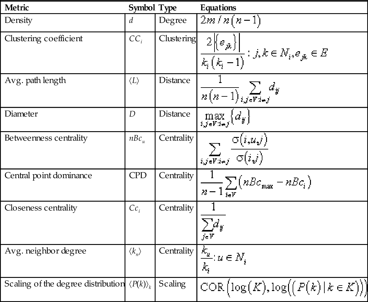
i,j,k,u∈V represent vertices, n, number of nodes; m, number of edges; k_i, degree of i; N_i is the neighbors of vertex i; e_jk, edges connecting the neighbors j, k of i; d_ij, length of the shortest path between i, j; σ(i, u, j)_, number of shortest paths between i and j that pass through u; σ(i, j)_, total number of shortest paths between i and j; nBc_max, maximum vertex betweenness; COR(X, Y), Pearson correlation coefficient between tuples X and Y; K, tuple of different vertex degrees in G; log(S), function that returns a set with the logarithm of each element in the set S.

• Degree metrics. Directly derived from the degree of vertices k_i and the degree distribution P(k). An example is the graph density d.

• Clustering metrics. The clustering coefficient CC_i is an example of a clustering metric that measures the cohesiveness of the neighbors of a node.

• Distance metrics. The average path length 〈L〉 is a well known distance metric. The diameter D of a graph, another well known distance metric, is defined as the length of the longest shortest path in G.

• Centrality metrics. Centrality metrics try to quantify the intuitive idea that some vertices and edges are more “important” than others. A popular example is the vertex betweenness centrality nBc_u that measures the proportion of shortest paths in which a vertex participates. The central point dominance CPD evaluates the importance of the most influential node in terms of the maximum betweenness centrality. The closeness centrality of a vertex i, Cc_i is inversely proportional to the sum of the distances of i to every other vertex in the graph.

• Scaling metrics. The presence of high-level properties of complex networks, such as the scale-freeness or the presence of a hierarchy of clusters, can be determined by observing the log-log plot of the scaling of local metrics with the degree of vertices. For example, the scaling of the degree distribution with the degree k, 〈P(k)〉_k can reveal the power-law nature of a graph.

Table 2 shows evidence that many of the metrics used for the study of complex networks could be redundant [7,22–25]. Metrics correlation patterns are dataset-specific and are affected by topological aspects such as the graph size, degree distribution, and density. The reader can refer to the mentioned works to find metrics correlations on graphs from different application domains.

Table 2

Works on Correlation Patterns on Complex Network Metrics

References	Complex Networks	Observations
[7,21,22]	Random, technological, social, biological, and linguistic.	Sets of highly correlated metrics are presented. Do not consider that some of the studied metrics are size-dependent.
[7]	Erdös-Rényi, Barabási-Albert, geographic networks.	Correlations patterns for individual network datasets do not agree with the correlations when the datasets are combined.
[23,24]	Erdös-Rényi, Barabási-Albert, autonomous system networks.	Metric correlations are affected by the degree distribution. Correlation patterns change with the size and density of graphs.
[25]	Erdös-Rényi, random modular, random hierarchies, US airlines, Wikipedia networks.	Warn against mixing network ensembles from different domains to extract global metric correlation patterns. Size-dependent metrics distort the correlations between metrics.

The algorithms to calculate most of the distance and centrality metrics listed in Table 1, such as the betweenness centrality, the closeness centrality, the average path length, and the central point dominance, are all based on BFS searches.

These distance/centrality metrics are computing intensive. Their calculation in large sparse graphs involves many full BFS traversals, resulting in hours to months of processing in modern CPU architectures if parallelism is not exploited, or if repeated measurements are needed.

The computational cost of BFS-based complex network metrics and the size of real-world networks stress the necessity for parallel approaches that exploit modern hardware architectures. The following section is devoted to this issue.

5.4 Efficient Complex Network Traversal

BFS is an intuitive search strategy that discovers the vertices of a graph by levels. Starting from a given vertex, BFS visits all the vertices at distance 1 from that vertex, then all the vertices at distance 2, and so on.

BFS represents an important core in a variety of complex network applications. BFS-based centrality metrics, such as the betweenness centrality, have been used, for example, to identify key proteins in protein interaction networks [26], and to identify the most relevant agents (leaders and gateways) in terrorist social networks [27]. Additionally, the betweenness centrality appears as a kernel of the HPC scalable graph analysis benchmark. Likewise, both the Graph500 and GreenGraph500 benchmarks include a kernel that consists of the repetition of BFS on huge networks.

However, even when a single BFS takes only On+m time, the mentioned applications need to perform an elevated number of BFSs (i.e., as many as the number of vertices in the graph). This is called AS-BFS. AS-BFS needs On2+nm time, where n can range from thousands to billions of nodes. The computational cost a variety of BFS applications on complex networks reveal the need for parallel strategies that exploit the features of modern HPC hardware architectures, in order to speed up the analysis of large and evolving networks.

5.4.1 HPC Traversal of Large Networks

Multicore processors have few yet complex processing units or cores with an on-chip hierarchy of large caches for general purpose and HPC processing. HPC clusters, a type of distributed memory architecture, is a group of workstations or dedicated machines connected via high-speed switched networks optimized for computing intensive large-scale calculations.

There is a list of publicly available libraries that exploit homogeneous parallel processing, (i.e., the use of a single HPC parallel architecture, such as a multicore server or a HPC cluster). Examples of such libraries include the Small-World Network Analysis and Partitioning (SNAP) library [28], The MultiThreaded Graph Library (MTGL) [29], the Parallel Boost Graph Library (PBGL) [30], the ParallelX Graph Library (PXGL) [31], and the Combinatorial BLAS library [32].

A GPU is a special-purpose HPC processor composed of many multithread cores. GPUs were initially designed as graphics accelerators for the PC and video game industry. Nowadays, GPUs are being used to accelerate a wide variety of scientific algorithms. Its popularity has increased since GPUs offer massive parallelism, huge memory bandwidth, and a general-purpose instruction set.

Most of the current GPU-accelerated BFS algorithms (e.g., [33–38]) are visitor/level-synchronous; each level is visited in parallel, preserving the sequential ordering of BFS frontiers [36]. Some works change the queue data structure to either increase locality or decrease intralevel synchronization overhead [35,36]. Other works avoid using a queue frontier structure by exhaustively examining nodes [34] or edges [38] in the current frontier, or by a warp-centric programming method [39]. Finally, there are works that try to reduce the number of traversed edges [33] and to reduce the interlevel synchronization overhead [35,40].

However, current results show that it has been difficult to leverage the massive parallelism of GPUs to accelerate the visitor approach on real-world graphs [34–36]. Speedups heavily depends on the graph instances, and there are real-world instances where the GPU implementation is slower than its CPU counterpart [34,35]. The performance of level-synchronous strategies is strongly influenced by topological properties, such as the diameter [36,39] or the degree distribution (due to load imbalance on SF graphs).

Sparse matrix operations provide a rich set of data-level parallelism, which suggest that algebraic formulations of BFS, based on sparse matrix-vector multiplications (SpMVs), might be more appropriate for the GPU data-parallel architecture [37,41]. Even when SpMV is considered a challenging problem due to the insufficient data locality and the lack of memory access predictability on real-world sparse matrices [37,42], it still offers higher arithmetic loads and clearer data access patterns than the classical visitor approach. In the following sections, we further discuss the use of GPUs for accelerating AS-BFS by describing and comparing two algorithmic approaches: visitor and algebraic (SpMV) AS-BFS.

5.4.2 Algorithms for Accelerating AS-BFS on GPU

There are two levels of parallelism that may be appropriate for GPUs: (1) medium-grain: for each BFS frontier, the exploration of all vertices in the frontier can proceed totally in parallel; and (2) fine-grain: for each BFS frontier, the exploration of the edges that go from the current frontier to the next one can be traversed in parallel. In this section, we describe two level-synchronous algorithmic approaches for AS-BFS that exploit these two different levels of parallelism on GPU: (1) visitor AS-BFS and (2) SpMV AS-BFS.

For the visitor BFS, we describe the GPU strategy reported in [38], which exploits both fine- and medium-grain parallelism. This efficient dual parallelism strategy leads to load balance even on SF graphs [38]. For the SpMV AS-BFS, we describe a two-phase strategy: SpMV and then zero-counting. The SpMV approach is also efficient on SF graphs. Both strategies perform frontier-wise synchronization with kernel relaunching, in such a way that each kernel launch triggers the exploration of the next BFS frontier.

Algorithms 1 and 2 show the pseudocode of the visitor AS-BFS strategy on GPU, first proposed in [38]. The vector l stores the distance between the source vertex and every other vertex by using the number of the current BFS frontier. Starting from every vertex s∈V, Algorithm 1 invokes the visitor kernel on GPU as many times as the number of BFS frontiers.

Algorithm 1 1GPU-visitor algorithm (host)

Algorithm 2 Visitor kernel (GPU)

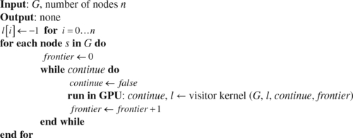
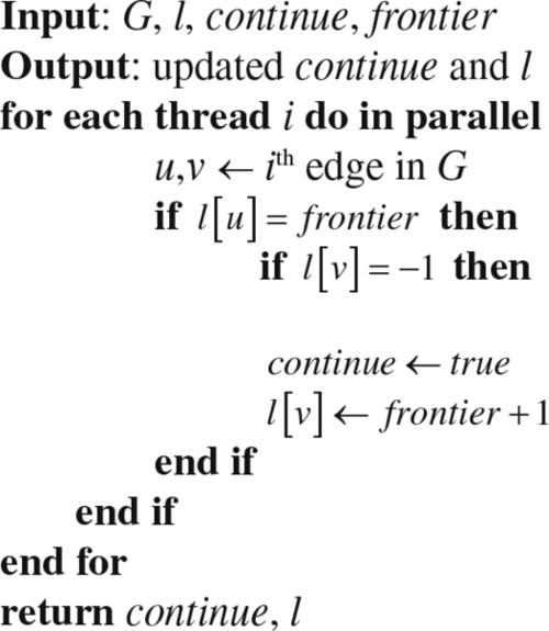
Algorithm 2 shows the pseudocode of the GPU kernel for the concurrent examination of all edges in the current BFS frontier. In each kernel invocation, all the edges of G are distributed among the GPU threads. Each GPU thread then examines if its edge connects the current BFS frontier to the following frontier. If so, it raises a flag (continue) to indicate that there is a new BFS frontier that must be explored in the following kernel invocation.

Algorithm 3 shows a pseudocode for the medium-grain SpMV AS-BFS on GPU. As the reader may notice, the strategy is very similar to the visitor algorithm for GPU: We perform a full BFS from each vertex s∈V, sequentially. However, in this case we accelerate the SpMVs and the zero-counting on GPU.

Algorithm 3 GPU-SpMV algorithm (host)

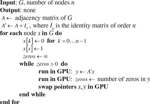
Then, we simply interchange the device pointers of the x and y vectors, so that we can reuse the allocated space and intermediated data produced in the device during the whole AS-BFS calculation. Algorithms 1 and 3 have no output, as they only show how to traverse the graph.

5.4.3 Performance Study of AS-BFS on GPU’s

We study the performance of the described GPU AS-BFS algorithms by comparing them to multithreaded (MT) CPU implementations. To make a comprehensive study, we experimented by varying the topology (degree distribution P(k) and density d) of synthetic regular and non-regular complex network-like networks.

To simulate different graph loads, we made use of the classical Gilbert and the Barabási-Albert random graph models, which allowed the creation of random graphs with exponential decay (Exp) and SF degree distributions, respectively. For the regular graphs, we experimented with the r-regular graph model (graphs where every vertex is connected to r other vertices).

For each degree distribution (Exp, SF and regular), we generated a dataset of very sparse (d∈0.0006,0.003) and sparse (d∈0.003,0.006) graphs with 40,000 vertices; and a dataset of dense (d∈0.01,0.5) and very dense (d∈0.5,1) graphs with 3,000 vertices. In spite of the difference in the number of vertices between the two datasets, the number of edges is comparable (up to around 4 M edges).

We implemented the MT visitor and the SpMV AS-BFS algorithms in a straightforward fashion, by uniformly distributing the single-source BFSs at random among the available cores. Both the MT and the GPU implementations were compared to a baseline sequential CPU visitor AS-BFS implementation.

The GPU visitor/SpMV experiments ran on a NVIDIA C2070 (Fermi) GPU with 448 CUDA cores at 1.15 GHz and 6 GB GDDR5 of DRAM. The multicore visitor/SpMV experiments ran on AMD Opteron 6274 (Interlagos) processors at 2.2 GHz and 64 GB of RAM, by using 16 cores. The sequential CPU visitor experiments ran on the same CPU architecture, but by using only a single core.

Fig. 1 summarizes the best speedups among the MT and GPU implementations over the sequential visitor approach, averaged over very-sparse, sparse, dense, and very-dense nonregular (Exp and SF) and regular graphs.

Fig. 1 Comparison of speedups between the multicore and GPU AS-BFS implementations over a single-core CPU visitor implementation, on graphs with different densities and degree distributions. In the non-regular column, “Exp.” stands for “exponential” and “SF” stands for “scale-free” degree distribution.

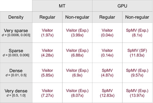
Fig. 1 shows that the visitor approach is better suited for CPU multicore, whereas the SpMV approach is better suited for GPUs. On the other hand, it can be seen that GPUs are not suitable for regular sparse graphs: both SpMV and visitor approaches performed poorly on GPU (sequential CPU was 25 times (very sparse) and 7 times (sparse) faster than GPU visitor).

Gain of GPU over sequential CPU increased with the graph density. With larger amounts of edges comes larger workloads that can exploit the massive multithreading capabilities of this architecture for performing parallel SpMVs. Overall, the best speedup over sequential CPU was obtained with the SpMV GPU implementation on very dense graphs.

We observed that structural properties present in complex networks influence the performance of level-synchronous AS-BFS strategies in the following (decreasing) order of importance: (1) whether the graph is regular or nonregular, (2) the graph density and (3) whether the graph is SF or not. Note that CPUs and GPUs are suitable for complementary kinds of graphs. GPUs performed notably better on sparse graphs. This is in contrast to multicore CPUs, which performed better than GPUs on regular graphs.

These results suggest that the processing of BFS on large real-world graphs could benefit from a topology-driven heterogeneous computing strategy, that combines CPUs and GPUs in a single heterogeneous platform by considering the presented empirical evidence of the suitability of a variety graph loads to different parallel architectures.

5.5 k-Core-Based Partitioning for Heterogeneous Graph Processing

Heterogeneous computing seeks to divide a compute intensive task into parts that can be processed separately by different parallel architectures in a synchronized manner. The ultimate goal of heterogeneous computing is to maximize the data processing throughput of an application by executing computing intensive part of an algorithm in accelerators, usually in a GPU [43].

Two major strategies for graph heterogeneous computing processing are [44]: (1) heterogeneous switching and (2) heterogeneous partitioning. In heterogeneous switching, the computation switches among different architectures according to a scheduler policy. The scheduler determines if the data can be better processed by another device. In heterogeneous partitioning, the computation proceeds in parallel on two or more parallel architectures at the same time.

Table 3 shows heterogeneous computing works for a variety graph problems (e.g., BFS, PageRank, connected components) that present different combinations of parallel architectures, including: CPU + GPU, CPU + APUs, and CPU + MICs.

Table 3

Works on Heterogeneous Computing of Graphs

References	Architectures	Architectures	Algorithm(s)	Partitioning
[45–47]	CPU + GPU	Heterogeneous partition	BFS, PageRank	Node degree
[48]	CPU + GPU	Heterogeneous switching	BFS	Frontier size
[44]	CPU + APU	Heterogeneous partition and heterogeneous switching	BFS, PageRank	Node degree
[49]	CPU + GPU	Heterogeneous partition and heterogeneous switching	BFS	Architecture memory bandwidth
[50]	CPU + GPU	Heterogeneous partition	BFS, connected components, all pairs shortest paths	Not specified
[51]	CPU + MIC	Heterogeneous switching	BFS	Frontier size
[52]	CPU + GPU	Heterogeneous switching	BFS	Frontier size

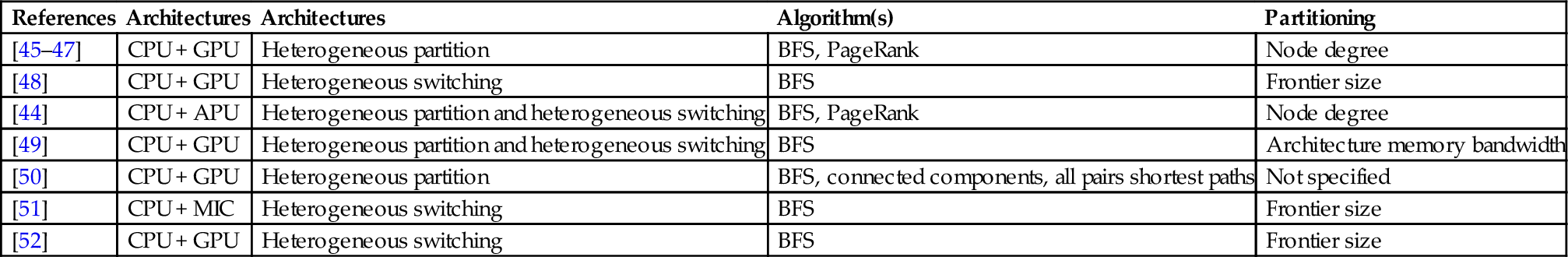
The last column lists the graph topological aspects used as criteria for partitioning the complex networks.

The first problem faced by any heterogeneous computing platform is to decide the best way to partition the load for later distribution among the available processors. Most existing graph partitioning algorithms produce equivalent partitions of the graph nodes [53], i.e., the produced partitions have a balanced number of nodes and the crossing links are minimized. In heterogeneous computing, however, the computing capabilities of the available processors varies, as do the size and properties of the scheduled tasks.

According to [45,46], a good graph partitioning strategy for heterogeneous computing should have: (1) low space and time complexity, (2) the ability to handle SF graphs, (3) the ability to handle large graphs, and (4) focus on the reduction of computation time.

In this section, we tackle the problem of graph partition for graph heterogeneous computing as an important step towards the efficient traversal of large graphs on heterogeneous HPC platforms.

5.5.1 Graph Partitioning for Heterogeneous Computing

It is possible to render communication overhead negligible in kernels like BFS and PageRank on SF graphs by exploiting aggregation techniques and a BSP parallel model [45,46]. As a consequence, the graph partitioner does not need to minimize the communication time, and it should instead focus on producing partitions that minimize computing time [45,46].

Partitions should offer two levels of parallelism: (1) a heterogeneous level to maximize the utilization of the processors, (2) and a homogeneous level to balance the workload across the vertices of a partition [45,46]. A simple criteria for distributing the vertices among the parallel processors is the vertex degree. Placing high-degree vertices in the CPU and low-degree vertices in the GPU [45,46] provides homogeneity of the nodes placed in the GPU, and minimizes GPU thread divergence as well [44]. This intuitive strategy also leads to partitions that are cache-friendly, an important property for memory-bounded algorithms like BFS [44–46]. Finding a bisection that splits the graph into two partitions with very different vertex degrees helps to leverage the computing power of CPUs and GPUs when combined into a single heterogeneous platform [44,45,47].

In Section 5.4.3, we showed that graph density is an important factor that affects the suitability of graphs to parallel architectures. Density, in addition to homogeneity, needs to be considered when partitioning a graph. There is evidence that complex networks are integrated of: (1) a dense partition of well-connected vertices and (2) a comparatively larger, sparse and homogeneous partition of low-degree vertices [54]. How can we exploit this property to identify the vertices that belong to the dense area of a complex network?

5.5.2 k-Core-Based Complex-Network Unbalanced Bisection

The k-core of a graph is its largest subgraph whose vertices have degree at least k [55] and can be calculated efficiently by recursively pruning the vertices with degree smaller than k in O(m) time. The concept of corenness is a natural notion of the importance of a node. For example, it has been reported that autonomous system networks show a “core” [54], integrated of highly connected hubs that represent the backbone of the Internet. The k-core decomposition defines a hierarchy of nodes that allow us to differentiate between core and noncore components of a network.

Vertices at the highest k-cores are located in the network’s densest area, the area that maintains the clustering structure of the graph. Thus, the k-core decomposition represents a useful yet easy to calculate heuristic for deciding which vertices belong to the dense partition and which vertices belong to the sparse one.

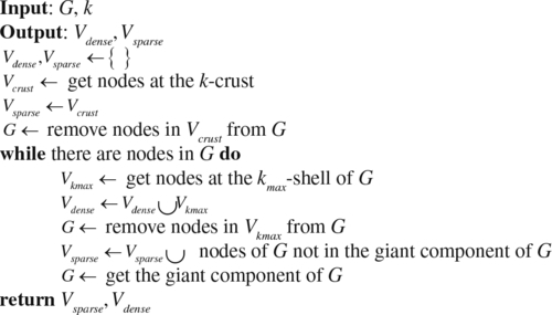
The authors propose the KCMax heuristic [56], listed in Algorithm 4, to produce a graph bisection algorithm that exploits the notion of k-core decomposition. The main idea behind the KCMax approach is: by repeatedly extracting the core of the network, we can separate the dense area of the network from the sparse one.

Algorithm 4 KCMax graph bisection

This separation would produce an unbalanced bisection of the graph that can be exploited for load distribution on heterogeneous platforms.

Formally, a k-core of a graph G=V,E is a subgraph H=C,L|C, induced by the set C⊆V, if and only if ∀v∈C:kv≥k and H is a maximum subgraph with this property. The k-cores are nested, i.e., i<j→Hj⊆Hi, like Russian nested dolls [57]. The k-crust is the graph G with the k-core removed. A node v∈V is said to belong to the k-shell if and only if it belongs to the k-core but not to the k+1-core. We say that if v is in the k-shell then v has a shell index of k.

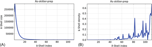
The KCMax algorithm starts by appending to the sparse partition, V_sparse, the nodes located at the k-crust of the graph. Then, it removes the k-crust from G. This preprocessing step is motivated by the fact that the k-crust nodes are unlikely to belong to the dense partition of the graph as they are very likely to hold a low clustering degree (Fig. 2). In practice, a large percentage of nodes in complex networks can be readily assigned to the sparse partition and removed from the graph to speed up the algorithm.

Fig. 2 Decomposition of the AS-Skitter graph. Horizontal axis shows the k-sell index. The vertical axis shows: (A) the number of nodes inside each k-shell and (B) the density of the subgraph induced by each k-shell. Note how most of the nodes belong to the least-dense k-shells. These nodes can be readily assigned to the sparse partition in a preprocessing stage to accelerate the KCMax heuristic.

The search for the dense area begins by identifying the nodes at the highest nonempty k-shell, the k_max-shell. Then, it appends the vertices at k_max-shell to the list of nodes in the dense partition, V_dense. The nodes at k_max-shell are removed from G, and only the giant component of G is retained for the next iteration. The nodes that are not in the giant component are assigned to the sparse partition, V_sparse. The algorithm repeats this procedure until the graph is depleted and all the nodes have been assigned to either the sparse or the dense partition.

The objectives of keeping the giant component after removing the k_max-shell are: (1) to help the heuristic to focus on the connected component that is more likely to contain clusters of nodes, and (2) to help the heuristic to reduce the number of iterations by discarding small components that result from the removal of the highest shell.

Table 4 lists large complex networks from a variety of application domains partitioned by exploiting the KCMax heuristic. Most of the graphs are real-world complex networks, with the exception of the R-MAT Graph500 synthetic graph. roadNet-PA, a road network of Pennsylvania, is unique in its large diameter and very low clustering (the small-world property is not present).

Table 4

Complex Network Dataset

Graph	Type	n	m	〈CC〉	D
AS-Skitter	Internet	1,696,415	11,095,298	0.2581	25
soc-LiveJournal1	Social	4,847,571	68,993,773	0.2742	16
cit-Patents	Citation	3,774,768	16,518,948	0.0757	22
com-orkut-ungraph	Social	3,072,441	117,185,083	0.1666	9
soc-pokec-relationships	Social	1,632,803	30,622,564	0.1094	11
R-MAT	Synthetic	388,317	16,777,184	0.1996	ND
roadNet-PA	Road	1,088,092	1,541,898	0.0465	786
Wiki-Vote	Vote	7115	103,689	0.1409	7
Email-Enron	Email	36,692	183,831	0.4970	11
Cit-HepPh	Citation	27,770	352,807	0.3120	13

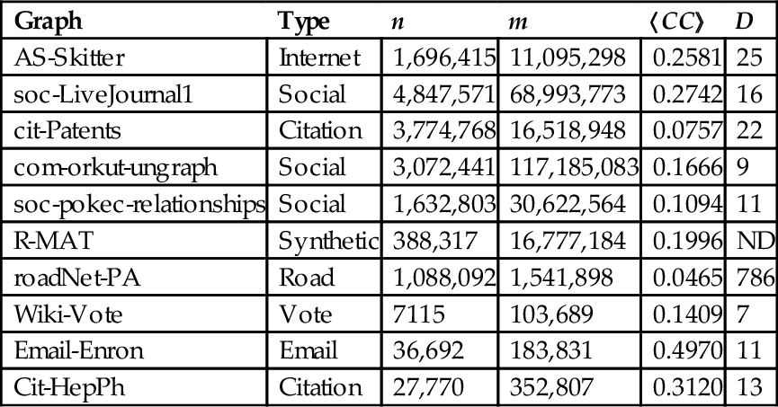
n, number of nodes; m, number of edges; 〈CC〉, avg. clustering coefficient; D, diameter; and ND, no data.

Tables 5 and 6 present the properties of the produced sparse and dense partitions, respectively. Note that, in general, the sparse partition concentrates more than the 50% of the vertices. In the AS-Skitter, soc-LiveJournal1, and cit-Patents graphs, the sparse partition accounts for more than the 90% of vertices.

Table 5

Properties of the Sparse Partition Produced by KCMax

Graph	n	∑​ki	d	c	Avg. deg.
AS-Skitter	1,565,489 (92.38%)	11,041,869 (49.76%)	2.17×10−6	242,272	7.05
soc-LiveJournal1	4,687,387 (96.77%)	59,300,536 (69.20%)	2.35×10−6	182,963	12.65
cit-Patents	3,641,824 (96.75%)	28,351,467 (85.85%)	2×10−6	18,396	7.78
com-orkut-ungraph	2,365,979 (77.01%)	94,072,948 (40.14%)	1.13×10−5	68,191	39.76
soc-pokec-relationships	909,797 (55.72%)	5,999,391 (13.45%)	1.76×10−6	360,457	6.59
R-MAT	286,526 (73.80%)	2,278,227 (7.67%)	1.46×10−6	226,227	7.95
roadNet-PA	214,395 (19.71%)	260,233 (8.44%)	1.99×10−6	168,628	1.21
Wiki-Vote	4595 (65.03%)	18,246 (9.06%)	5.09×10−5	4062	3.97
Email-Enron	26,011 (77.19%)	92,145 (25.48%)	4.36×10−5	16,375	3.54
Cit-HepPh	11,060 (32.15%)	82,111 (9.76%)	7.02×10−5	7051	7.42

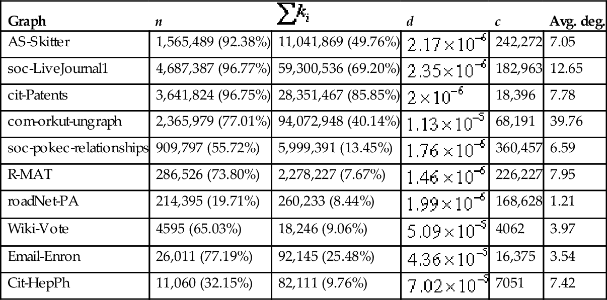
n, nodes; ∑​ki, sum of the degrees of the vertices in the partition; d, density of the graph induced by the partition; c, number of components in the graph induced by the partition; and avg. deg., average degree of the vertices in the partition.

Table 6

Properties of the Dense Partition Produced by KCMax

Graph	n	∑​ki	d	c	Avg. deg.
AS-Skitter	129,127 (7.62%)	11,146,549 (50.24%)	3.2×10−4	2	86.32
soc-LiveJournal1	156,566 (3.23%)	26,390,832 (30.80%)	7.6×10−4	12	168.56
cit-Patents	122,293 (3.25%)	4,672,013 (14.15%)	1.9×10−4	12	38.20
com-orkut-ungraph	706,462 (22.99%)	140,297,218 (59.86%)	2.2×10−4	1	198.59
soc-pokec-relationships	723,006 (44.28%)	38,604,537 (86.55%)	6.51×10−5	1	53.39
R-MAT	101,711 (26.20%)	27,413,457 (92.33%)	2.4×10−3	1	269.52
roadNet-PA	873,167 (80.29%)	2,822,795 (91.56%)	3.48×10−6	3	3.23
Wiki-Vote	2471 (34.97%)	183,226 (90.94%)	2.72×10−2	1	74.15
Email-Enron	7685 (22.81%)	269,477 (74.52%)	3.5×10−3	5	35.06
Cit-HepPh	23,341 (67.85%)	759,457 (90.24%)	1.25×10−3	2	32.53

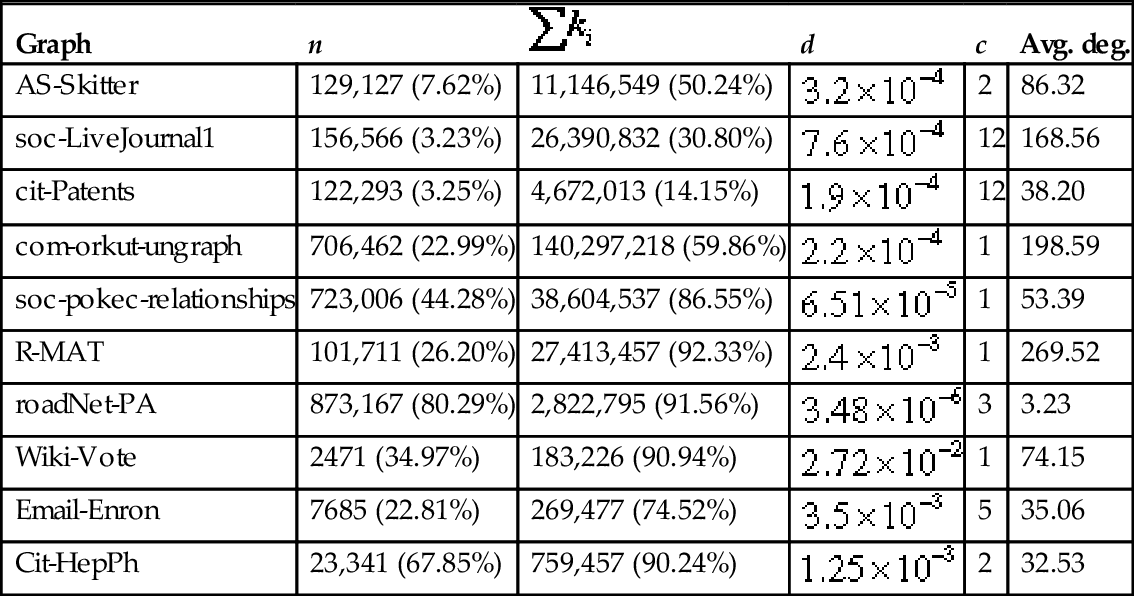
n, nodes;∑​ki, sum of the degrees of the vertices in the partition; d, density of the graph induced by the partition; c, number of components in the graph induced by the partition; and avg. deg., average degree of the vertices in the partition.

Likewise, note that in complex networks, a small proportion of vertices in the dense partitions concentrates a high number of edges. Take as examples the Email-Enron network, where 22.81% of the vertices are connected by 74.52% of the links; the R-MAT network, where the 26% of the vertices are connected by 92% of the links; and the Wiki-Vote network, where the 34% of the vertices are connected by 90% of the links.

In some complex networks, a degree of balance between the sparse and the dense partitions arises, either in the number of nodes or in the number of links. For example, in the soc-pokec-relationships and Wiki-Vote networks the 55% and the 65% of the vertices are assigned to the sparse partition, respectively; whereas in the AS-Skitter and com-orkut-ungraph networks the 49% and 40% of the links are assigned to the sparse partition, respectively.

The dense partition of most of the experimented graphs is several orders of magnitude denser than the sparse partition. An exception was the roadNet-PA, whose partitions showed the same order of density. In all graphs, however, the density of both the sparse and the dense partitions was relatively low.

Finally, note that the dense partitions are generally composed of at most a dozen of connected components, while the sparse partitions are composed of thousands of connected components. Additionally, the average degree of the vertices in the dense partition is one order of magnitude larger than in the sparse partition in virtually all graphs (with the exception of roadNet-PA, where it is two orders of magnitude higher). The remarkable difference in the number of components, the density and the average degree in the partitions suggest that KCMax was able to locate those vertices that integrate the densest part of the graphs in all cases.

5.6 Future Directions

The processing of AS-BFS-related algorithms on large real-world graphs can exploit a topology-driven heterogeneous computing strategy, that combines CPUs and GPUs by considering the presented empirical evidence shown in Section 5.4.3 of the suitability of a variety graph loads and algorithms to different parallel architectures and different BFS algorithms approaches.

The authors have observed that Totem [45–47], a graph computation framework that exploits single-node multicore + GPU heterogeneous systems, can benefit from the KCMax partitioning heuristic [56]. Other projects that follow a BSP-like parallel computational model and that focus on minimizing the computation time of partitions could take advantage of the partitions produced by the KCMax algorithm as well.

Future work include: (1) the extension of the KCMax algorithm to calculate an arbitrary number of partitions by recursively applying the KCMax heuristic to the bisection, in order to provide support, for example, to multi-GPU architectures; and (2) producing a graph library that exploits a variety of BFS kernels accelerated by different hardware architectures, while hiding the heterogeneous computing workload distribution details from the user for the acceleration of traversal-based complex network applications.

5.7 Conclusions

Network science and complex network are becoming increasingly relevant for representing and analyzing multi-relational Big Data and in modeling complicated data structures and their interactions. The main idea behind a complex network is to model high-order interactions among the individual components of large systems by means of graphs, to increase our understanding of not only immediate but also high-order interactions, as well as the implications of these interactions on the mechanisms that govern the underlying phenomenon.

We presented algorithms for performing HPC traversals on large sparse graphs by exploiting CPU multicores and GPUs. By comparing the visitor and algebraic BFS approaches, we showed that structural properties present in complex networks influence the performance of AS-BFS strategies in the following (decreasing) order of importance: (1) whether the graph is regular or non-regular (2) whether the graph is dense or not, and (3) whether the graph is SF or not. In addition, we showed that CPU’s and GPU’s are suitable for complementary kinds of graphs.

Finally, we described the KCMax graph bisection heuristic, that capitalizes on the notion of k-core decomposition to identify and separate the dense area of a complex network from the sparse one. This separation would produce a bisection of the graph where each partition is suitable for different parallel architectures, that can be exploited for load distribution on parallel heterogeneous platforms. We partitioned a collection of large real-world graphs and showed the properties of the partitions induced by the bisection.

Ongoing work includes the adaption of the unbalanced graph partitioning algorithm KCMax to BSP-like heterogeneous platforms, to minimize computation time instead of communications, and accelerate the traversal and calculation of BFS-based metrics on big real-world networks, with the objective of overcoming the limitations of homogeneous platforms.

References

[1] Committee on Network Science for Future Army Applications. Network science. Washington, DC: National Academies Press; 2005.

[2] Lima M. Visual complexity, 2015. http://www.visualcomplexity.com/vc/ [accessed 01.07.15].

[3] National Center for Biotechnology Information. Growth of GenBank and WGS, 2015. http://www.ncbi.nlm.nih.gov/genbank/statistics [accessed 25.10.15].

[4] Facebook. Facebook reports first quarter 2015 results. Menlo Park, CA: Facebook; 2015 http://investor.fb.com/releasedetail.cfm?ReleaseID=908022; [accessed 25.10.15].

[5] WorldWideWebSize.com. The size of the world wide web (the internet), 2015. http://www.worldwidewebsize.com [accessed 25.10.15].

[6] Joseph I., Vodenska E., Stanley E., Chen G. Netconomics: novel forecasting techniques from the combination of Big Data. Netw Scie Econ. 2014 arXiv:1403.0848.

[7] Costa L.F., Rodrigues F.A., Travieso G., Boas P.R.V. Characterization of complex networks: a survey of measurements. Adv Phys. 2007;56(1):167–242.

[8] Guida M., Maria F. Topology of the Italian airport network: a scale-free small-world network with a fractal structure? Chaos Solitons Fract. 2007;31(3):527–536.

[9] Angeloudis P., Fisk D. Large subway systems as complex networks. Phys A Stat Mech Appl. 2006;367(15):553–558.

[10] Yazdani A., Jeffrey P. Complex network analysis of water distribution systems. Chaos. 2011;21(1):016111.

[11] Robinson I., Webber J., Eifrem E. Graph databases. Boston, MA: O'Reilly Media; 2013.

[12] Neo4j. The world's leading graph database, 2015. http://www.neo4j.org [accessed 01.07.15].

[13] OrientDB, OrientDB graph-document NoSQL DMBS, 2015. http://www.orientdb.org [accessed 01.07.15].

[14] Objectivity. InfiniteGraph, 2015. http://www.objectivity.com/products/infinitegraph/ [accessed 01.07.15].

[15] Malewicz G., Austern M.H., Bik A.J.C., Dehnert J.C., Horn I., Leiser N., et al. Pregel: a system for large-scale graph processing. In: Proceedings of the 16th international conference on management of data (COMAD'2010), Indianapolis, USA, June 6–11; 2010.

[16] Giraph. Welcome to Apache Giraph! http://giraph.apache.org [accessed 01.07.15].

[17] Hassibi K., Dean J. High performance data mining and Big Data analytics. New York: Wiley; 2012.

[18] Lumsdaine A. Challenges in parallel graph processing. Parallel Process Lett. 2007;17(1):5–20.

[19] Sharma P., Khurana U., Shneiderman B., Scharrenbroich M., Locke J. Speeding up network layout and centrality measures for social computing goals. In: Proceedings of the 2011 international conference on social computing, behavioral-cultural modeling and prediction; 2011.

[20] Strogatz S.H., Watts D.J. Collective dynamics of 'small-world' networks. Nature. 1998;393(6684):440–442.

[21] Filkov V., Saul Z.M., Roy S., D’Souza R.M., Devanbu P.T. Modeling and verifying a broad array of network properties. Europhys Lett. 2009;86(2):28003.

[22] Jamakovic A., Uhlig S. On the relationships between topological measures in real-world networks. Netw Heterogen Media. 2008;3(2):345–359.

[23] Garcia-Robledo A., Diaz-Perez A., Morales-Luna G. Correlation analysis of complex network metrics on the topology of the internet. In: Proceedings of the 10th international conference and expo on emerging technologies for a smarter world, Melville, USA, October 21–22; 2013.

[24] Li H.W., de Haan W., Stam C.J., Van Mieghem P. The correlation of metrics in complex networks with applications in functional brain networks. J Stat Mech Theory Exper. 2011;2011(11):P11018.

[25] Bounova G., de Weck O. Overview of metrics and their correlation patterns for multiple-metric topology analysis on heterogeneous graph ensembles. Phys Rev E. 2012;85(1):016117.

[26] Koschützki D., Schreiber F. Centrality analysis methods for biological networks and their application to gene regulatory networks. Gene Regul Syst Biol. 2008;2(1):193–201.

[27] Yang C.C. Knowledge discovery and information visualization for terrorist social networks. In: Chen H., Yang C.C., eds. Intelligence and security informatics: techniques and applications. Philadelphia, PA: Springer; 2008.

[28] Madduri K. A high-performance framework for analyzing massive complex networks. PhD thesis Atlanta, GA: Georgia Institute of Technology; 2008.

[29] Berry J.W., Hendrickson B., Kahan S., Konecny P. Software and algorithms for graph queries on multithreaded architectures. In: Proceedings of the 21st IEEE international symposium on parallel and distributed processing (IPDPS'2007), Long Beach, USA, March 30; 2007.

[30] Gregor D., Lumsdaine A. The parallel BGL: a generic library for distributed graph computations. In: Proceedings of the 5th workshop on parallel/high-performance object-oriented scientific computing, Glasgow, UK, July 25; 2005.

[31] Stark D. Advanced semantics for accelerated graph processing. PhD thesis Baton Rouge, LA: Louisiana State University; 2011.

[32] Buluç A. Linear algebraic primitives for parallel computing on large graphs. PhD thesis Santa Barbara, CA: University of California; 2010.

[33] Beamer S., Asanovic K., Patterson D. Direction-optimizing breadth-first search. In: Proceedings of the 2012 ACM/IEEE international conference for high performance computing, networking, storage and analysis, Salt Lake City, USA, November 10–16; 2012.

[34] Harish P., Narayanan P.J. Accelerating large graph algorithms on the GPU using CUDA. In: Proceedings of the 14th international conference on high performance computing, Goa, India, December 18–21; 2007.

[35] Luo L., Wong M., Wen-Mei H. An effective GPU implementation of breadth-first search. In: Proceedings of the 47th design automation conference, Anaheim, USA, June 13–18; 2010.

[36] Merrill D., Garland M., Grimshaw A. Scalable GPU graph traversal. In: Proceedings of the 17th ACM SIGPLAN symposium on principles and practice of parallel programming, LA, USA, February 25–29; 2012.

[37] Qian H., Deng Y., Wang B., Mu S. Towards accelerating irregular EDA applications with GPU's. Integr VLSI J. 2012;45(1):46–60.

[38] Shi Z., Zhang B. Fast network centrality analysis using GPU's. BMC Bioinform. 2011;12(149):1–7.

[39] Hong S., Kim S.K., Oguntebi T., Olukotun K. Accelerating CUDA graph algorithms at maximum warp. In: Proceedings of the 16th ACM symposium on principles and practice of parallel programming, San Antonio, TX, February 12–16; 2011.

[40] Liu G., An H., Han W., Li X., Sun T., Zhou W. FlexBFS: a parallelism-aware implementation of breadth-first search on GPU. In: Proceedings of the 17th ACM symposium on principles and practice of parallel programming, New Orleans, USA, February 25–29; 2012.

[41] Kepner J., Gilbert J. Graph algorithms in the language of linear algebra. Philadelphia, PA: Society for Industrial and Applied Mathematics; 2011.

[42] Goumas G.I., Kourtis K., Anastopoulos N., Karakasis V., Koziris N. Performance evaluation of the sparse matrix-vector multiplication on modern architectures. J Supercomput. 2009;50(1):36–77.

[43] Gelado I., Stone J.E., Cabezas J., Patel S., Navarro N., Hwu W.W. An asymmetric distributed shared memory model for heterogeneous parallel systems. In: Proceedings of the 15th edition of architectural support for programming languages and operating systems (ASPLOS’2010), New York, USA, March 13; 2010.

[44] Nilakant K., Yoneki E. On the efficacy of APUs for heterogeneous graph computation. In: Proceedings of the 4th workshop on systems for future multicore architecture, University of Cambridge, UK; 2014.

[45] Gharaibeh A., Santos-Neto E. Efficient large-scale graph processing on hybrid CPU and GPU systems. J Supercomput. 2013;71(4):1563–1586.

[46] Gharaibeh A., Costa L.B., Santos-Neto E., Ripeanu M. On graphs, GPU's, and blind dating: a workload to processor matchmaking quest. In: Proceeding of the 2013th international parallel and distributed processing symposium, Boston, USA, May 20–24; 2013.

[47] Gharaibeh A., Costa L.B., Santos-Neto E., Ripeanu M. A yoke of oxen and a thousand chickens for heavy lifting graph processing. In: Proceedings of the 21st international conference on parallel architectures and compilation techniques, Minneapolis, MN, USA, September 19–23; 2012.

[48] Hong S., Oguntebi T., Olukotun K. Efficient parallel graph exploration on multi-core CPU and GPU. In: Proceedings of the 2011 international conference on parallel architectures and compilation techniques, Washington, DC, USA, October 10–14; 2011.

[49] Zou D., Dou Y., Wang Q., Xu J., Li B. Direction-optimizing breadth-first search on CPU-GPU heterogeneous platforms. In: Proceedings of the 10th IEEE international conference on high performance computing and communications and 2013 IEEE international conference on embedded and ubiquitous computing, Zhangjiajie, November 13–15; 2013.

[50] Banerjee D.S., Sharma S., Kothapalli K. Work efficient parallel algorithms for large graph exploration. In: Proceeding of the 20th annual international conference on high performance computing, Bangalore, India, December; 2013.

[51] Gao T., Lu Y., Zhang B., Suo G. Using the Intel many integrated core to accelerate graph traversal. Int J High Perform Comput Appl. 2014;28(3):255–266.

[52] Munguia L.M., Bader D.A., Ayguade E. Task-based parallel breadth-first search in heterogeneous environments. In: Proceedings of the 19th international conference on high performance computing, Pune, December 18–22; 2012.

[53] Chamberlain B.L. Graph partitioning algorithms for distributing workloads of parallel computations. Seattle, WA: University of Washington; 1998 Technical report.

[54] Carmi S., Havlin S., Kirkpatrick S., Shavitt Y., Shir E. A model of internet topology using k-shell decomposition. Proc Nat Acad Sci USA. May 2007;104(27):11150–11154.

[55] Dorogovtsev S.N., Goltsev A.V., Mendes J.F.F. K-core organization of complex networks. Phys Rev Lett. 2006;96:040601.

[56] Garcia-Robledo A., Diaz-Perez A., Morales-Luna G. Exploring the feasibility of heterogeneous computing of complex networks for Big Data analysis. In: Proceedings of the 12th international conference and expo on emerging technologies for a smarter world, Melville, USA, October 19–20; 2015.

[57] Batagelj V., Zaversnik M. An O(m) algorithm for cores decomposition of networks. Adv Data Anal Classi. 2003;5(2):129–145.