Packing Algorithms for Big Data Replay on Multicore
Abstract
This chapter discusses optimization in a new environment created as an alternative to Hadoop/MapReduce. The core idea is to bring the bulk from now-passive shard nodes to a dedicated machine and replay it locally while a large number of jobs are running on multicore. This chapter discusses optimization methods for machines with a large number of cores and processing jobs. This chapter also discusses how the new architecture can easily accommodate advanced Big Data-related statistics, namely streaming algorithms.
Keywords
Packing algorithms; Big Data replay method; Massively multicore; Hadoop; MapReduce; Data streaming
10.1 Introduction
This chapter discusses the Big Data Replay approach to processing Big Data. Given that Hadoop [1] coupled with MapReduce are the current de facto standards in this area, the replay method reviewed in this chapter is the direct rival and alternative to the current de facto standard.
The core replay method was first introduced in Ref. [2] where the architecture of Hadoop [1] is discussed in detail and compared with the new, replay-based architecture. It presented only a crude idea of relay, while this chapter goes in depth and focuses on the various ways in which the replay method can be optimized in relay. As the title of this chapter says, the replay environment is assumed to be multicore — in fact, this chapter introduces the new concept of massively multicore — which creates many interesting challenges when trying to optimize the entire environment. In fact, Hadoop/MapReduce also attempts to optimize its resources, as well as access to them, but does it in a distributed manner, while the replay method in this chapter offers a diametrically opposing viewpoint by performing all the activities on a single, massively multicore machine.
This chapter is not the first to discuss Hadoop/MapReduce alternatives. Based on the clearly recognized performance limits of Hadoop [3] — this article is, in fact, written by one of the current developers of Hadoop — there are calls for alternative technologies (see Ref. [4]) with bold titles that yet send a clear message.
For clarity a, let us simplify the terminology. In reality, Hadoop — or the Hadoop Distributed File System (HDFS) — is an independent technology from MapReduce. The latter is, in fact, an algorithm that can be implemented by Big Data processing engines to run jobs on Hadoop. Recent software packages implement several engines other than MapReduce, which means that Hadoop/MapReduce logic is no longer true. HDFS itself is challenged by several new distributed file systems — see Ref. [3] for a short overview. However, for simplicity, let us use the term Hadoop to refer to both a distributed file system and an engine that runs jobs on it. By far, the current de facto technology is Hadoop/MapReduce, but this could change in the future. Given the drastic difference between any Hadoop technology and the one-machine environment discussed in this chapter, it is likely that the difference in performance shown in this chapter can be applied to newer distributed engines. From this point on, the term Hadoop will always mean any distributed file system and job execution engine.
Hadoop performance has already been modeled [5] and analyzed statistically [6] — such research has shown that there are solid limitations to the throughput, both in terms of the file system changes and job execution performance. Several parts of Hadoop have also been improved, creating a different tool. For example, there is an attempt to exploit multicore hardware on shards (a storage node on a Hadoop cluster is referred to as a shard). More traditional research would try to optimize the job schedule in order to maximize the overall utility of the system. There are more peculiar studies that add a structured metadata layer to the otherwise unstructured Hadoop shards, using R in Ref. [7] and Lucene indexing in Ref. [8].
The biggest improvement, however, is only possible via a drastic change of the research scenery. This change is discussed in the form of the distributed versus one-machine argument in Ref. [4]. In fact, the related argument is that the distribution is a curse, which has been admitted by the creators of Hadoop [3], but this discussion normally does not lead to a solid conclusion. Instead, even the paper that presents the one machine is better argument says that the one-machine environment is only for relatively small data bulks, while Hadoop remains the only choice for true Big Data.
There is a large body of literature on the various optimizations of the traditional Hadoop. Name nodes are recognized as single points of failure (SPOF), but a system that allows for multiple name nodes has to tackle new challenges related to the need for synchronization across the nodes and the increased overhead between the now multiple name nodes and shards.
A great deal of research work is entirely dedicated to optimizing job execution shards. For example, the Tiled MapReduce method [9] is a standard partitioning approach from parallel programming applied to the jobs competing for resources at the same shard. However, such research does not optimize the entire Hadoop system because each job is run on multiple shards, and optimizing each shard separately does not necessarily result in optimal performance for the entire system.
Returning to the one-machine theme, while it has been mentioned in Ref. [4], the context is very different from the technology discussed in this chapter. The context in Ref. [4] is that the bulk is lower than 10–15 GB, in which case it can be handled on the commodity hardware of a single machine. However, no assumptions are made on the multiple jobs, multicore architecture, and various other components discussed in this chapter.
The correct one-machine theme is the Big Data replay method itself [2]. The immediate difference from the idea in Ref. [4] is that the engine can easily scale up to any bulk size. But the more important difference is that the machine is assumed to be multicore — even massively multicore, if possible — which allows for the variable scale in terms of the jobs running in parallel. Although the logic of the replay method is different from the traditional Hadoop, it is expected that the scale of 10 k parallel jobs can be reached on each replay node — multiple nodes can also be used without any major increase in overhead. However, the correct method for evaluating the replay method is to measure the job throughput as the number of jobs per unit of time, in which case, depending on the unit of time, the overall throughput of the system can easily exceed the 10 k level of the current Hadoop.
This chapter uses the core replay method, but focuses specifically on the packing algorithms applied to multiple parallel jobs. The new focus requires several new components, some of which can be found in recent literature, some of which come from this author. Efficient parallelization in the lockfree shared memory design is discussed in Ref. [10] in a traffic-specific version which can be easily generalized and applied to Big Data. Data streaming [11] is offered as the main framework for jobs and, as such, replaces the key-value datatype used by MapReduce [12]. Data streaming can support any kind of a complex datatype, for example many-to-many structures are discussed in Ref. [13] and one-to-many (referred to as superspreaders) in Ref. [14]. There are the various algorithms and efficiency tricks in data streaming [15], but the most important feature is that data streaming algorithms are normally implemented along the timeline and require that a time window be input into the data [16]. Finally, this chapter will discuss the recently introduced circuit emulation technology which is used for bulk data transfer [17] — this research area is known as Big Data networking. The core idea of Big Data Replay was presented in Ref. [2] and early prototypes and demos in Ref. [18].
The actual contributions of this chapter are as follows: on top of the basic replay method in Ref. [2], this chapter assumes massively multicore hardware. There is a clear distinction between massively multicore and manycore, explained in detail further into this chapter. With the high number of cores, this chapter focuses on packing algorithms. The jobs are packed into batches, each having its own time window. The main job of the runtime optimization engine is to optimize the batches. The two specific models formulated and analyzed in this chapter are Drag and Drop, each referring to an approach to dealing with the gradual scattering of time cursors of individual jobs in each batch. The various parameters of the replay environments, however, offer a rich space which can support several other models, as well as several versions of the two main models.
10.2 Performance Bottlenecks
A very good overview of the various HDFS/MapReduce bottlenecks can be found in Ref. [3]. Some are reviewed and repeated in this chapter, but the scope in this chapter is considerably larger and includes separate consideration of storage (Hard Disk Drive (HDD)/Solid State Drive (SSD)) and shared memory (shmap) performance bottlenecks. Shared memory in this chapter is shortened to shmap, which is the name of the most efficient/popular library used in multi- and manycore systems today. This section presents experimental data for these two components which become datasets in analysis later in this chapter.
10.2.1 Hadoop/MapReduce Performance Bottlenecks
Fig. 1 shows the primitive viewpoint at performance bottlenecks, which will be upgraded twice throughout this chapter. The bottlenecks are divided into network, storage and shared memory types, each with its own relative width — the pipe analogy here assumes that wide pipes have bigger bottlenecks and therefore offer better performance.
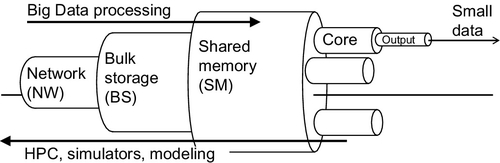
Network is the narrowest bottleneck and indicates strong and well-recognized performance problems. The base parameters are delay, throughput, and variation of both [13]. These parameters are very hard to predict and/or control, and become increasingly more so as multiple traffic flows compete for resources. Traditional Hadoop is a good example of a networking environment where very many small and large traffic flows complete for bandwidth.
Bulk storage is represented by HDD/SSD disk. They make shards in traditional Hadoop. In replay, storage can be used for temporary on-disk caching of bulks brought in from remote storage nodes. This bottleneck is actively discussed in the research. For example, one of the issues is the HDD versus SSD problem, where it is a widely spread myth that SSD is better than HDD, but there is also research that shows that a hybrid optimization engine can outperform either of the two technologies [19].
Shared memory bottlenecks depend on the capacity offered by shmap libraries among several offered in modern kernels [20]. Capacity can be improved by drastically reducing the overhead from locking and message passing when using the lockfree design [10]. Shared memory is a hot discussion topic in multi- and manycore parallel programming. Technical advice on code generation can be found in Ref. [21]. Advanced research in this area makes a clear distinction between hardware and software support, as well as between multi- and manycore systems [22]. Message passing interface (MPI) technology has recently been shown to perform the best when implemented after the lockfree design (one-side communication), based on shared memory [23].
Jobs on cores themselves are also bottlenecks. This time, the capacity is mostly affected by the computing load itself. For example, as Fig. 1 shows, the processing job is supposed to convert Big Data to Small Data, which requires complex processing logic, state, etc. This chapter will reveal an interesting revelation by showing that the overhead in jobs is the biggest contributor to overall performance degradation. Still, the batch management methods and packing algorithms presented further in this chapter can help elevate this problem, up to a given degree. The problem cannot be eliminated completely since processing data is the fundamental necessity of both Hadoop and Replay engines.
Note that Fig. 1 shows the fundamental difference between Big Data processing and high performance computing (HPC). Here, the shift from multi- to manycore systems advertised in Ref. [22] is applicable only to the HPC part as such research needs to build more and more powerful supercomputers. However, it is unlikely that the Big Data part of the research will move in the same direction. For example, manycore systems are not good for moving large bulks of data quickly — in fact, the main purpose of HPC is to generate data using modeling, simulation, etc. Since the process in Big Data processing is the inverse of that, the networking bottleneck is extremely important — it is like having a very small entrance into a very large stadium. Using the same analogy, HPC tries to build larger stadiums because it focuses on what is happening inside the stadium and pays little attention to what gets in and out of it — thus not paying much attention to the networking bottleneck. This is changing, however, in recent literature, which has finally come to terms with intercluster networking in manycore clusters and started to look for technologies that can improve the situation. Circuit emulation, discussed later in this chapter, is applicable here as well.
There are several smaller bottlenecks. The various software and logic bottlenecks are discussed in Refs. [3] and [4]. For example, it is shown that only 75% of traffic to the name node can be dedicated to job traffic, while the rest is overhead. HDFS write/read limits are known to be 55/45 MB/s, respectively. Various other overheads can cause bottlenecks in replication, job management, etc.
However, there are also bottlenecks which are not considered in Ref. [3] and are generally left without attention in programming-related areas. For example, traffic contention and congestion can cause drastic differences in performance [10], especially when very small lookup/metadata flows compete with the flows that carry the bulk of job results. The circuits in Ref. [17] cover just that fact. This general discussion is revisited several times in this chapter, and specifically when discussing the hotspot distribution (bulk flows in traffic can be classified as hotspots).
Even smaller bottlenecks are created by unfair competition across jobs, especially when the load is heterogeneous [5,6]. This is a recognized problem, and several ways to resolve the problem are being looked into — for example, the tool in Ref. [24] is a scheduler of heterogeneous jobs. The key-value output datatype for MapReduce jobs is too restrictive and creates a bottleneck for jobs. This problem is addressed in Ref. [4], where it is mentioned that the only way to counter this issue is to run multiple Hadoop rounds. The true resolution is discussed in this chapter, which advocates for the general data streaming framework for processing jobs, which offers the complete freedom of datatypes [12]. The same bottleneck is created by the lack of time awareness on Hadoop [4]. This is also countered by running multiple rounds of jobs, but can be fundamentally resolved via the data streaming approach. Note that using a free datatype is difficult on Hadoop, but is trivial on the one-machine environments such as those discussed in this chapter.
10.2.2 Performance Bottlenecks Under Parallel Loads
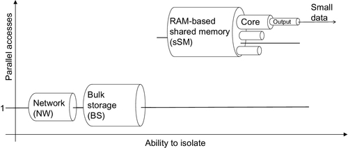
Fig. 2 adds more dimensions to the problem. In fact, the simple bottlenecks presented in the previous subsection should be examined from the viewpoint of
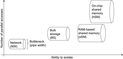
– ability to isolate a user of a resource from other parallel users
– the number of parallel users for a given resource
both applied to each separate bottleneck discussed herein.
Both of the two new parameters affect the performance (width) of the bottleneck. For example, an initially large bottleneck can be reduced if it cannot be properly isolated, and is subjected to many parallel clients, where both metrics are found at work at the same time. This, in fact, refers to the shmap experiment found later in this section.
The network is the hardest technology to isolate. See the argument against network virtualization in Ref. [25]. The good news is that not much parallel access to network resources is happening in the one-machine environment under the replay method. However, by extension, this is also the weak point of the traditional Hadoop, which subjects this initially weak/narrow bottleneck to very high-count parallel loads. Recently, the same problem has been recognized in manycore systems as well [22], and recent research has started to look for ways to optimize the load for minimizing traffic between clusters. Even further, the same problem, although to a lesser extent, occurs inside the manycore clusters. The replay method offers another advantage — the replay node can use circuits to transfer the bulk from a remote node for local replay [17].
Disk and traditional shmap are found somewhere in the midrange of the two axes in Fig. 2. The traditional view in terms of storage is that SSD is better than HDD, but this viewpoint is wrong. First, the difference depends on the type of use. Second, when a generic use is intended, recent literature has shown that hybrid optimization — hybrid meaning that the storage has both HDD and SSD in it — performs better than either of the two technologies separately [19].
Comparing storage and shared memory, one has to keep in mind that there are far fewer parallel accesses to the storage than to shmap. Taking the job batches later in this chapter as an example, the difference is obvious — parallel access to storage relates to the number of batches, while parallel access to shared memory is much higher because all the jobs in batches also have to access the shmap library in parallel. The experiment and dataset later in this chapter reveal the practical outcome of such a difference.
The on-chip shmap version in Fig. 2 requires special attention. This is the special case in manycore systems which implement L1 and L2 caches on the chips themselves and supports them by hardware and software. A good description of the advantages of such an upgrade is offered in Ref. [22]. Modern manycore systems offer many efficiency tricks which drastically improve performance, and therefore, increase the size of the bottleneck. Yet, congestion from parallel access can affect performance even in such advanced systems [23].
10.2.3 Parameter Spaces for Storage and Shared Memory
The two further subsections in this section offer the actual experimental data and datasets related to storage (SSD) and shared memory (shmap) performance. This subsection serves as the introduction by presenting the parameter space and the related terminology for the two experiments.
Fig. 3 shows the parameter space for the two technologies as well as the connection between the two (dotted lines). The rest of this subsection is dedicated to explaining this parameter space.
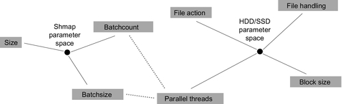
Shmap is defined by
– size, denoting the size of the RAM memory dedicated to shared memory
– batchcount denoting the number of parallel batches, each batch having its own shmap space
– batchsize denoting the number of jobs running in a batch and, therefore, sharing the individual shmap for that batch
Note that this space already offers a clear view of the situation with parallel access. One might be tempted to think that only batches compete in parallel. In reality, both batch managers and all the individual jobs in all batches are the processes running on top of the same kernel and, as such, are competitors for the same shared resource. The competition within the batch can be minimized by using the lockfree design discussed herein. The only way to avoid the competition for the globally shared kernel attention is to separate the batches physically. Manycore systems, in a way, are the tool for physical separation between cores and core clusters. The framework discussed in this section assumes that the same will be attempted in future generations of multicore hardware, hopefully leading to massively multicore hardware architectures.
Storage performance is defined by
– file action, referring to what you do with a file, specifically read, write or append, etc.
– file handling, which refers to how the file is handled in the long run — where the two obvious alternatives in massively parallel systems are to keep file handles open continuously or reopen files for each batch; later experiments will also use the seek parameter for denoting whether or not the reading position in the file has to change for each new/next time window
– blocksize, denoting the size of the chunk in each read/write operation within each session
– finally, parallel threads denotes how many threads/processes are using the storage in parallel
The connection between the two parameter spaces is obvious and relates to the parallel aspects of the two technologies. The term parallel threads in storage relates to batchcount, and batchsize is shmap. The relationship is a bit subtle, however, since only the batchcount equals the number of parallel accesses to storage, while batchsize further contributes to the overall competition in the shmap domain.
The two remaining subsections in this section run experiments and construct datasets for these two parts.
10.2.4 Main Storage Performance
This subsection presents the first of the two experiments — those that target the storage performance. The HDD versus SSD argument was discussed in the previous section, but for simplicity, the experiment is run only on the SSD storage. In fact, the shmap experiment described later in this chapter will show that the storage bottleneck is minor by comparison, which means that the HDD versus SSD argument, as well as the hybrid optimization with the combination of the two, will not offer a tangible increase in the overall performance of a Big Data Replay engine.
The following experimental design is used: only read operations are used — the multiGB files from which the reading is done are created in advance. Otherwise, the file handling methods are complex, and include the combination of
– the openeach versus keep file handling method, where the former refers to a method in which the file is closed after each batch and reopened for the next, and keep, naturally, refers to the opposite method
– seekeach versus continue, which refers to whether or not to call on a the seek() system call to change the reading position within the file or continue from the last (or initial) position
In the aftermath of the experiments, there was a realization that the parameters had relatively little effect on the overall performance. Instead, the blocksize parameter and the number of parallel threads had the greatest effect.
The code for the experiment was written in C/C++. The parallel threads were, in fact, implemented as separate processes. In fact, the terms thread and process are used interchangeably in this chapter, unless a distinction is clearly denoted in a given context. For the majority of cases, modern operating systems do not make a tangible distinction between the two. The experiment was run on a commodity 8-core (Intel i7) hardware platform.
Each experimental round was conducted as follows: first, all the threads/processes are spawned, but are designed to start at a future time — each thread monitors the global time and starts at roughly the same time as all the others. Once started, each thread/process opens the file once and then makes 10 iterations of the reading operation with the preceding parameters. For each iteration, the file can be closed and reopened, seek() can be used to change the reading position, but the blocksize of bytes is read in all iterations, resulting in the total bulk of 10 times the blocksize.
Since the experiment is conducted with the idea of creating a practical dataset, detailed measurements are taken by each thread. Each one records the time for each stage of reading in each iteration, resulting in open, seek, and read values for each iteration. In addition, each thread outputs the final took in total value that measures the time it took the thread to complete all 10 iterations. As the figures later in this subsection show, the final figure is not always the sum of the figures from individual iterations.
Fig. 4 shows the raw JSON [26] output of one of the experimental runs. The two blocks are for light (above) versus heavy (below) setups. The header has all the parameters, while the bottom part has the curtailed version of the data for each thread in the parallel pool. The first line is the legend, while all the other lines show the values for individual threads.
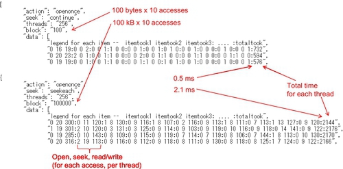
The following observations can be made from the raw output. In the light version (above) there are many 0 values in individual threads. This is to be expected and has to do with clock resolution. Since reading a very small block of data can be really fast, the kernel might have had no time to update the clock during the operation. Another way to put it is to say that no context switching was performed during that simple operation — this explanation is not strictly true, but is adequate for most practical cases. The total time (last number) for each thread still reflects the adequate time — this value is used when creating the dataset based on the raw data.
The heavy use at the bottom of Fig. 4 shows that the time increases by a factor of about 3. Values for individual iterations are also now adequate because it takes a much longer time to read 100 kB from the file. Same as before, the final number (total time) is used to put together the dataset.
Fig. 5 illustrates the entire dataset constructed for many experiments covering the entire parameter space, with two or more states for each parameter. Specifically, up to 512 threads (processes) and blocks from 100 bytes to 100 kB were used. The visualization method in Fig. 5 is a 2D representation of the multidimensional data. The image is cast into 2D by presenting the results in a flat sequence of all the combinations of parameter values. The most important factor in such visualizations is the order of parameters — depending on the order, the resulting visualizations can range from those that are very easy to read to those that make no sense entirely. The order selected in Fig. 13 — action, threads, block, seek — is assumed to be easy to read. Since action and seek have a minimal effect on the overall performance, various other orders can result in the same rough view as long as the threads and blocks parameters are in that order.
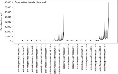
Fig. 5 shows that the number of threads and blocksize are the two largest effects. Blocksize arguably has a greater effect, which is evident from rapidly growing peaks — this parameter is the last in the iteration loops. However, the threads parameter also plays its role, which is evident from the two islands of peaks in the visualization. Note that the values on the vertical scale are the actual completion times. Since the blocksize is known, one can easily use the image to calculate the practical throughput of the reading operations at a given setting.
10.2.5 Shared Memory Performance
The second experiment is for shmap. The same commodity hardware is used; this time the important system parameter is the 4 GB of RAM, which is more than enough to cover the needs for all the parallel batches.
The experiment was conducted as follows: the parameter space was used exactly as was presented in an earlier subsection — the parameters are size, batchcount, and batchsize. As before, the threads are orchestrated by defining a starting time in the future. This time, the logic is a little bit more complex because separate starting times have to be defined for managers of batches versus processing jobs. It was found that it was sufficient to start managers at 2 s in the future, which is enough time for them to write the shmap before individual jobs starting at 5 s can start reading each of their own batch’s shmap individually. As before, the software was written in C/C++, using the standard shmap library [20].
Fig. 6 is the raw JSON output, this time for the shmap experiment. The raw output is again split into light (above) versus heavy (below) parts. Each record has the header with parameters and the body of performance data (curtailed to several lines) where the first line is the legend. This time, each line in the data represents performance aggregated for a given batch. The design of each line (see the legend) accounts for that by showing the time it took for the manager thread to create and populate the shmap and then add all the reading times for individual job threads. The practical use of this data is also slightly different. The completion time of the batch is defined as open plus write plus the largest of the read times among the jobs. Simply put, this means that the batch ends only when the slowest job has finished reading and processing the content of its shmap. This feature is revisited later when the topic of heterogeneous loads is discussed, resulting in job packing logics which take the related problems into account.
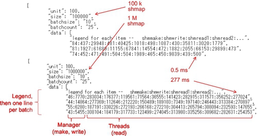
Let us see what stands out in the raw data. The only difference between the light and the heavy runs is the size of the shmap — it changes from 100 k to 1 M. The scale — defined as batchcount times batchsize — is the same for both experiments. However, we see a huge difference in raw numbers between the upper and lower parts. This effect was confirmed from raw data and the software was tested extensively to make sure that the effect was there.
Let us judge the difference in performance. In the light version, the majority of reading times are in 3 digits, some are 4, and only a few are 5 digits long. The heavy data, however, is mostly populated by 6-digit numbers, representing a decrease in performance by a magnitude of 3
The following conclusions can be drawn from raw performance. The ability to isolate RAM appears to be lower than that of storage. Obviously, both the parallel access and size of shmap have an effect on performance, but, judging from the raw data in Fig. 6, increasing the size of shmap can have a major effect by itself.
Fig. 7 offers a 2D visualization of the entire dataset. Since the size has the largest effect, the order is size, batchcount, batchsize. The following simple interpretation of the visualization can be offered. When the size is small, the other two parameters have little effect. However, when the size of shmap is large, both batchcount and batchsize start to have a major effect on performance, starting at the midrange of the values.
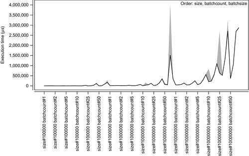
This chapter will use the dataset in its current form while future research will focus on finding more details on the aforementioned drastic difference in performance.
10.3 The Big Data Replay Method
This section explains the basics of the replay method and discusses the connection between time-aware processing of Big Data [16], specifically the data streaming approach [11], and the traditional Hadoop. This section also discusses recent advances in Big Data-related technology such as, for example, circuit emulation for bulk transfer. The section is concluded by a discussion of the various other performance bottlenecks which can happen in the new system.
10.3.1 The Replay Method
This section focuses on explaining the design of the architecture powered by the replay method. For comparison with Hadoop architecture see Ref. [2].
Fig. 8 shows the architecture of the basic replay method. The following major changes are introduced:
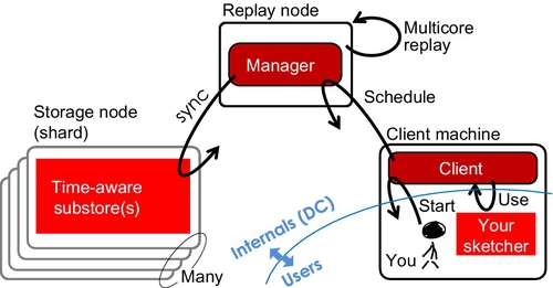
– Shards are dumb storage while Hadoop assumes that jobs are executed on shards; note that the storage in shards is time-aware because shards can be replayed along the timeline.
– The name node is replayed by the replay manager — although the two are functionally very different. The name node represent the most important node in a cluster; however, in the replay method there is no name service, instead the shards are replayed in accordance with their time logic (sync operation in the figure).
– Clients and users are not the same node anymore, instead, the user can be a remote machine used to schedule jobs on clients, which can be internal to the cluster (located inside DCs) — note the distinction of external versus internal traffic to the name node, as well as the contention between the two, which is a major problem in Hadoop.
The client/user part of the new design is an interesting element in itself. In data streaming, statistical digests of data are referred to as sketches [11]. The design in Fig. 8 borrows the term and shows that jobs can be implemented as sketches. Since sketches are statistically rigid (scientifically provable and mathematically defined), it is also likely that users would not come up with their own sketches, but would instead use a library provided at the client. This is another element where users and clients represent not only different roles, but also different physical machines.
Note that the intensive (meaning high-frequency) traffic exchange disappears both between clients and replay nodes as well as users and clients. Basically, only two exchanges are necessary — one to upload a sketcher and the other to download the results. Also note that the replay node does not strictly need to be multicore, but the presence of a multicore architecture greatly enhances the performance and flexibility of replay nodes. In fact, this entire chapter is dedicated to showcasing how efficient packing algorithms can help maximize both the capacity and flexibility of replay nodes.
The replay node is obviously a SPOF, just like the name node in Hadoop. However, this SPOF can be easily fixed by running multiple replay nodes and balancing between them. The difference between eplay node and name node is also fundamentally of a different nature — in the case of Hadoop the bottleneck is in the network part, where the high-rate and high-frequency traffic has to complete for the entrance into the name node. By comparison, the traffic contention in relay node is extremely rare, while jobs mostly compete for the multicore resource. In other words, upgrading the replay nodes can help with performance bottlenecks in replay, while the performance bottlenecks in Hadoop are mostly physical in nature.
10.3.2 Jobs as Sketches on a Timeline
Fig. 9 shows a more detailed representation of the replay method, this time naming the components of the new environment:

– Time-awareness is assumed for shards — it makes it possible to know which shard comes after which other shard, and, otherwise, facilitates the core replay process.
– A manager is necessary to manage each of the multiple batches, where each batch is based on a shared memory (shmap) region.
– Shared memory is shared between managers and multiple sketches, where the communication is assumed to be designed in a lockfree manner and should not require any locking or message passing.
– There is a global cursor allowing the manager to denote the now, here position in shared memory, as well as individual cursors for each sketcher/job; both are necessary and are used for one-sided communication (lockfree) where jobs can detect the change in data and the manager can detect completion of batches by individual jobs.
– Finally, jobs have a clearly defined lifespan, which is a major improvement from the traditional Hadoop.
The obvious advantages of the new design are as follows: there is a clear parallel between time window and shared memory, where the shmap region can be, literally, treated by each sketch/job as a time-aligned window into the data. While jobs used to run in isolation, but using the same shards, in the new design, jobs are grouped in batches, where all jobs in the same batch process the same time window into data. Both these features are, in fact, on the list of requirements for the new generation of Hadoop-like systems [4]. In traditional Hadoop, such logic can only be implemented as multiple rounds of Hadoop jobs [4], each round covering the entire bulk of data. Communication between rounds may require that some kind of state be kept across rounds — another feature not supported by traditional Hadoop.
10.3.3 Performance Bottlenecks Under Replay
“Circuits for bulk transfer” refers to the circuit emulation technology in Ref. [17]. It works both in Ethernet and optical networks, and relies on the cut-through mode available in any modern switching equipment, even the cheapest models [27]. A side note here is due on circuits versus multisource aggregation — the circuits are assumed to offer a much higher efficiency, while multisource aggregation is the technology for maximizing throughput in extremely unreliable networking — clouds and Peer-to-Peer (P2P) networks are used as examples in Ref. [28]. Another way to put it is to refer to circuits as the technology for achieving nominal physical throughput while multisource aggregation is the technology for squeezing out the maximum possible performance given the circumstances.
Fig. 10 returns to the bottleneck representation, but this time discusses new technologies which help improve performance with the aforementioned replay logic in mind.
Circuits assume that there is only one flow, and therefore, only one receiver thread/process. This explains why parallel access for storage in Fig. 10 is also at 1. This requires a minor change of design. Instead of requiring each manager to get its own shards from remote storage nodes, one process/thread can be given the schedule and put in charge of fetching the bulk of data and writing it into the respective shmaps. This is not difficult to implement in practice. On the other hand, one has to remember that the advantage of such a design is significant since even two parallel flows achieve worse network performance than two flows scheduled to be transmitted in sequence, without a time overlap.
Note that the shmap bottleneck discovered and discussed in the previous section is retained in the upgraded Fig. 10. This is bad news, because the dataset discussed herein shows that shmap is the worst performance bottleneck as it is hard to isolate, and since its performance degrades drastically with an increased parallel load. However, good news is possible here, as well, if batches are isolated physically using the experience from modern manycore clusters.
10.4 Packing Algorithms
This chapter expands on the basic replay method explained in the previous section and explains the various efficiency tricks which exploit the newly acquired flexibility in the new system. Specifically, the system has grown in scale, up to the level of a massively multicore architecture, reaching the area where the various packing algorithms discussed in this section finally find sufficient room for performance improvement.
10.4.1 Shared Memory Performance Tricks
Essentially there are two ways to use shared memory, specifically, the shmap library referred to in this chapter — memory map versus pointer exchange. This subsection explains the two methods in detail.
The Memory Map method does exactly what the name says — all the data exchanged between the multiple users of shmap is supposed to be stored in shared memory. This is the conventional method, and it is used by the majority of shmap-based software today. Obviously the biggest problem with the method is the static structure itself. Dynamic changes and some level of variability can still be supported, however, they come at the price of having to increase the size of shmap and reduce efficiency by leaving some areas of the memory unused. This problem grows in proportion to the amount of variability/variety found in the data. Conversely, this problem is nonexistent if all data has a fixed and standard size — in fact, memory maps are the preferred format for fixed-size data structures.
Let us translate the Memory Map method into Big Data processing. Each time window is a time-aligned collection of data items. Variable-size items are standard for Big Data, with a few exceptions, such as Twitter, where one can safely assume that the message size cannot exceed 140 bytes (just as an example). There are two ways to convert such data into a memory map. First, one can find the largest size among all items in the window and then record the number globally, using it as the fixed size of all items in the shared memory. This makes walking the data a very simple endeavor. Alternatively, one can develop a protocol for writing variable-size records, which will drastically improve space efficiency, but will hinder walking, as each item will have to be parsed lightly before the system can jump to the next one. Either of these methods is sufficient, but the first method (fixed size) is always the best choice when processing speed is the first priority, hence, the fundamental problem with the memory maps.
Pointer Exchange via shared memory is possible. The proof of concept for this method is shown in Ref. [10]. It works with C/C++ threads and is not easily portable. On the other hand, passing the pointers — also referred to as passing complex structures by reference across processes is a very tempting feature.
The following example can be applied to Big Data processing. Double linked lists (DLLs), as in Ref. [10], can be created by the manager and passed to all processing jobs. Each job would then walk the DLL, mostly using the next pointer in each item, until the now cursor is reached (timestamps in items can help here). This method can also resolve another issue of the Memory Map method — the issue of where to put the results? In fact, given that it is hard to predict how many records (and of which size) are created by each job, one would find it very difficult to find a practical solution. In traditional multicore programming, the outcome is stringified and recorded somewhere outside of the shmap. The outcome can be put back into shmap only if its size and count are known in advance, but even in this case, communication in the opposite direction would require some form of locking or message passing. This is another reason for storing the outcome outside of shmap even if its size and count are known in advance.
The lockfree trick has already been mentioned, but requires special attention [10]. The basic description of the method is to say that the specific design makes it possible to minimize or completely remove locks in shared memory. The next step after design is automatic code generation in compilers.
A good example of a lockfree design is the aforementioned DLL. This example can also help the manager thread to process the outcome of the multiple processing threads in each batch. Let us assume that the output of each job is also put in the form of a DLL. This means that all the current items are also found in it — some outcome items may be the result of processing multiple raw items in the data stream. Let us also make a conscious decision to move an output item to the head of the DLL on each update — this is a simple operation in DLL that involves reassigning points and does not require any copy, delete, and other time-consuming operations. When this process is executed over time, one can easily visualize that old items would gradually sink to the bottom (tail) of the DLL since all update items are immediately moved to the head. This opens up the obvious hole for the lockfree trick — the manager can simply look at the tail of the DLL (via the direct pointer) and remove the time-outed output items without any communication with the job responsible for populating the DLL.
There is some literature on code generation for multicore parallel processing [29–32], but all such literature always uses locks and message passage as a part of its automatically generated code. In other words, the code generated with such compilers definitely performs much better than a single-core code, but much worse than the code crafted using the lockfree features. Note here that not all algorithms can be lockfree, by nature. For example, graph-based calculations [33] need coordination across threads, which is difficult to make lockfree. The good news is that Big Data processing jobs have zero need for interjob coordination, and are therefore the perfect subject for massive multicore environments.
There is a small body of literature that focuses on shared memory performance and discusses the various forms of lock optimization. Direct shmap access with kernel support is discussed in Ref. [34]. Shmap-based MPI implemented as a true one-side communication is proposed in Ref. [23].
10.4.2 Big Data Replay at Scale
Fig. 11 is an upgrade of the basic concept of replay presented earlier to a massively multicore environment. The new feature is the concept of job management within each time window. Each time window is dedicated to a given batch of jobs, where multiple batches can run on each replay node at any given point in time.
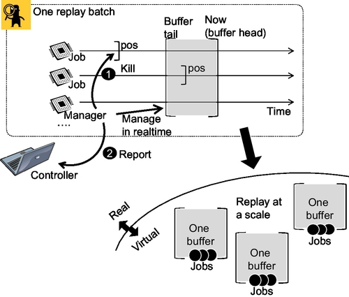
The physical versus virtual separation in the figure helps enhance the understanding of the nature of batches. The physical reality is that batches are shared memory regions and depend on lockfree designs [10], one-sided communication in MPI terminology [23], and the manager having to maintain the cursors for both the global position in the data and individual positions of processing jobs. However, the virtual representation allows for a simple abstraction which only keeps the elements required for the large-scale optimization of job packing. Which is why the simplified/virtual view only has batches and jobs allocated for each batch.
The virtual representation in Fig. 11 provides examples of the following problems. One problem involves packing a given number of jobs into a fixed number of batches — the traditional bin packing problem. Another problem involves transferring data too slow or too fast jobs between batches. Yet another problem can show how batches can be allocated in such a way that they would cover the largest possible span of time, in aggregate. The next subsection formulates the two most obvious packing algorithms. Future research will most likely reveal an expanded list of practical algorithms.
One main aspect to keep in mind when optimizing a scaled environment with many batches and many jobs is that jobs are heterogeneous. This means that one cannot know in advance whether or not a job can meet its expected timeline. The majority of attention focused on packing algorithms is spent on countering this very aspect. Heterogeneity of jobs is also covered in recent literature on multicore code generation [32], which contributes to the foundation for the generation of lockfree code in the future.
10.4.3 Practical Packing Models
Analysis described in the next section is performed based on the two practical packing algorithms. This subsection formulates each algorithm in detail.
The Drop algorithm represents the tough approach toward jobs management, hence its name. A batch is assumed to have a given fixed width (of the time window into data). The Drop algorithm would drop any job that goes beyond this width. The only alternative to dropping the job is to accommodate a larger window, which this algorithm avoids at all costs. Ideally, dropping a job does not result in that job’s destruction — it can be easily mapped to another batch or a newly created batch. In fact, the replay environment in this section is assumed to be extremely fluid and such dynamics are intended to be part of its normal operation. Likewise, a new job can be mapped to the current batch to replace the removed job, thus allowing for efficient use of batches and, ultimately, resources on replay nodes.
The Drag algorithm is the opposing strategy (to the Drop algorithm). It allows the time window of the batch to grow, thus accommodating all the initially assigned jobs without having to remove or reassign them. The good part of this strategy is that it saves the overhead from removing and reassigning jobs. However, the downside of this strategy is that the increasing time window means that batches take longer to complete or, in other words, the operational grain of the system increases. Also, in cases when only a single job is very slow compared to its neighbors in the batch, this strategy can lead to the overall inefficiency of the replay node. All in all, this strategy is intuitively inefficient, but is still used in analysis covered later in this chapter in order to provide the comparison with the Drop model, as well as to study the bounds of variability in batches.
There are, of course, various combinations of the two primitive algorithms described herein. For example, one can easily assume a hybrid algorithm, which allows the batch to grow up to a given point, after which it starts to drop jobs. When dropping the jobs, does one drop the fastest or the slowest job? In fact, in analysis described later in this chapter the dropping is done randomly at the head and tail, but a more rigid approach would probably look at the distribution of cursor times and remove the node (head or tail) which contributes the most to the variance.
10.5 Performance Analysis
Analysis in this section is based on the two datasets — for storage and shared memory — created and explained earlier in this chapter. The datasets enable trace-based simulation by supplying the real data for a given set of conditions. However, this section also adds the last components necessary for analysis — the hotspot distribution used to model heterogeneous environments. With this added component, simulations can now represent the full range of Big Data processing used in the replay method. The Drag and Drop models explained in the previous section are used as management routines for individual batches.
10.5.1 Hotspot Distributions
Hotspots [35] are normally used to describe extremely heterogeneous loads in a generic way. In numeric form, the distribution describes large populations of items, where a relatively small number of items contribute the overwhelming majority of the load.
The hotspots model was recently presented as a model for packet traffic [36]. The paper presents the mathematics behind the model, and the generation which can be applied both at packet and flow levels. A simplified version of the same method removes time dynamics and only uses sets of numbers [37].
The hotspot model is based on four sets of numbers referred to as normal, population, hot, and flash. In reality, there are only three sets, as hot and flash describe the same items at two different stages in their lifespans. The sets can be used to describe a wide range of heterogeneous phenomena occurring in nature. However, let us consider an example involving a content delivery network (CDN). In any CDN, the total number of hosted items is very large, but most of the items are rarely requested/watched — those are normal. The ratio of normal items can reach 80% in some cases; and higher with an increasing scale. A portion of the remaining items is watched more, but is not at the level of becoming hits — those are the popular items. The popular items rarely change during their lifespan — another way to describe it is a slow but steady demand for a given type of content (in CDN terminology).
The remaining hot/flash items are the core of the distribution. There are relatively few items, but they consume the majority of traffic to and from CDN. This happens because of two features hidden in the two sets. First, the level of hot popularity of an item can be sufficiently large and account for a major portion of traffic when the aggregate traffic with all the other hot items is considered. But, more importantly, hot items sometimes experience flash crowds — this is when the demand rapidly peaks for a given item — the value for this popularity comes from the flash set. The peak traffic can be sufficiently high to constitute the majority of CDN traffic on a given day.
In complex modeling, the process is modeled in time, allowing items to grow from hot to flash gradually. However, for the purposes of modeling in this chapter, the simplified version from Ref. [37] is applied, meaning that only the static sets are used without any time dynamics between them.
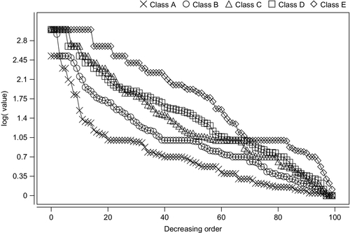
Yet, even in the simplified sets-only form, distributions are difficult to judge. It is helpful to classify distributions based on their curvature. The following classification method is applied in this chapter for the first time. First, imagine the log values of the sets plotted in decreasing order of value. Given the nature of the distribution, hotspots — there are normally only a few of them — would be plotted at the head of the distribution and then the curve would drop for the rest of the values. Note that the drop would be experienced even on the log scale. Here, the only way to classify such a distribution is to judge the size of its head.
So, classification in this chapter uses the following ranges for classification, all in log scale:
– if values at 80% and further into the list are 0.15 or above, then Class A is assigned
– if values at 60% and further into the list are 0.6 or above, then Class B is assigned
– if values at 40% and further into the list are 1.3 or above, then Class C is assigned
– if values at 30% and further into the list are 1.8 or above, then Class D is assigned
– if no class is assigned by this point, then Class E is assigned
The class preceding assignment is fine-tuned to the distributions used for analysis further in this chapter. The tuning was done in such a way that each class would get a roughly equal share of distributions, which were otherwise distributed for a reasonably large-parameter space. As another simplification, each hotspot distribution is converted into two separate curves by combining popular + hot and popular + flash sets, each classified and used separately. Only 100 values were generated for each distribution, but this is sufficient, as values during simulation are selected randomly from the list, which means that relatively low values are selected much more frequently than the large items. Otherwise, the same process is used as in Refs. [36] and [37], where there are 2–3 other parameters such as variance, number of hot items, variance across hot items, etc.
Fig. 12 shows several curves from the dataset, each marked in accordance with its calculated class. We can see that the classification is successful by assigning a higher letter to a curve with a relatively higher number of hotspots. Note that the generation process has no maximum value, but, in order to avoid extremely long processing sessions, all values exceeding 1000 are brought back to 1000. The values (not logs, but the original number behind) are translated into per-item processing time, expressed in microseconds (μs). To add more flexibility to the otherwise fixed pool of hotspot distributions, the scale parameter was added to scale per-item overhead within 1–3 orders of magnitude down from the value found in the hotspot dataset.
10.5.2 Modeling Methodology
Fig. 13 shows the overall simulation process, which puts the two real (storage and shmap) and one synthetic (hotpost) datasets into a single simulation.
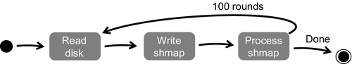
Simulation parameters come mostly from the two real datasets — one needs to set size, batchcount, batchsize for shmap, and threads, blocksize and others for storage. However, some simplifications are made at this stage. Blocksize is fixed to 100 k, in which 10 iterations makes for 1 MB, shmap is sized to 1 MB, and file handling is ignored as having little effect on performance. On the other hand, batchcount and batchsize are selected randomly from the values found in the dataset. Given that the two datasets are related, threadcount is not selected randomly but is set after the batchcount, based on the logical assumption that parallel storage handling is happening for all batches currently in operation.
The only new parameter added in this section is the class. The base hotspot classes were explained in the previous subsection. The parameter class can have values A, AB, ABC, ABCD, and ABCDE, randomly selected for each application. The values specify the range for classes during selection — for example, when set to ABC, hotspot distributions for each job in a given batch can be selected from any A, B, or C classes. In practical terms, this parameter controls the heterogeneity of jobs, where A class is the most and E class is the least heterogeneous.
Each simulation run is conducted in the order described in Fig. 13. Since the target is to emulate a real replay process on a massively multicore hardware, the simulation is built to closely mirror a real process. So, as Fig. 13 shows, first, the real dataset is used to emulate the storage operations — the stage at which, in reality, managers of shmaps read data from storage and use it to populate shmaps. Shmap population incurs additional overhead and is therefore isolated into a separate stage in the sequence. Finally, the contents of shmap are processed by all jobs in all batches, at which time the hotspot dataset (only the synthetic one) is used to model the additional overhead for each item on top of the baseline value spent by each job simply on reading the contents.
The scale parameter in simulation specifically targets this borderline between the baseline shmap reading and item-by-item processing. The baseline shmap reading time is used as the starting value for each job. However, the job is also expected to spend some time for each item found in shmap. For simplicity, items are considered to be 100-bytes long (10,000 items in the 1 MB shmap). To define the per-item overhead, each job selects a hotspot distribution (using the preceding class range) and selects values from it randomly, as processing time is in microseconds (μs), but also multiplying each value with the scale. The scale of 0.001 would basically mean that the largest (hotspot = rare) overhead is 10 μs, since the largest value in the hotspot datasets is 1000 μs. A scale of 1 would, therefore, describe cases where per-item overhead is extremely high.
The rest of this section will be dedicated to discussing the results of the simulation conducted using the preceding methodology.
10.5.3 Processing Overhead Versus Bottlenecks
One major element of this chapter is the bottleneck analysis, since removing or improving bottlenecks is the fastest way to improve the overall performance of the system. This subsection discusses a snapshot of aggregate simulation outcomes which clearly indicate where the performance bottlenecks are given the limitations of the system.
Fig. 14 aggregates all the outcomes for the simulations running with the setup of blocksize = 100 k (this is fixed for all), shmap size = 1 M (also fixed), batchcount = 10, and batchsize = 2 — this is a relatively light setting given that only 2 jobs are running in each batch. Note that scale, hotspot classes and other parameters are not part of the aggregation conditions, which means that the distribution curve contains all the outcomes from all the values in these and other parameters, which are not indicated in the selection rule (also plotted on the figure).
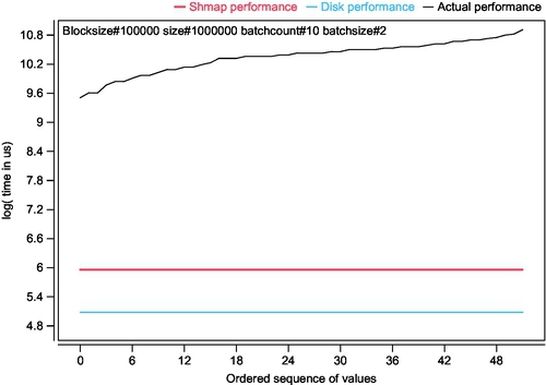
Before using this particular aggregation, the various selection rules were tested. Fig. 14 was found to be objectively better than all the other selection rules — this means that the lower end of the curve shows the best possible performance, that is, the one when the scale is set to 0.001, classes selected are the widest possible, etc.
So, Fig. 14 clearly shows that the per-item processing is, in fact, the biggest bottleneck in the system. By comparison, the shmap and disk/storage bottleneck are plotted as well — these values are the same for the selection rule. The term “bottleneck” can be confusing here because the horizontal lines represent completion time, that is, the reverse value to the width of the bottleneck. However, conceptually, the visualization concept still stands.
The simple take-home lesson from Fig. 14 is that, even given the shmap and storage performance bottlenecks, their effect can be neglected as long as the per-item processing performance remains at the shown level. Note that physical separation of batches as is done in manycore systems is not an option here. Also note that the 0.001 scale (between 0.001 and 10 μs per item overhead) might be too high for a realistic system, in which case the natural performance curve in some systems might be lower. Measurement of real loads as a subject is left for further study.
10.5.4 Control Grain for Drop Versus Drag Models
Fig. 15 presents several diagonal plots that compare performance between the Drop versus Drag packing algorithms. Note that performance metrics for the two methods are completely different. The Drop method is evaluated by the count of drops per unit of time. The Drag method does not allow for drops and can therefore be evaluated by the width of the time window after some running time. However, if the values are normalized, they can be compared in a diagonal plot. Here, the main target of the analysis is not to see the real values (10–20 drops versus 60–100 s windows were found in raw data), but to compare the distributions of values, where distribution curves can offer some insight into performance dynamics.
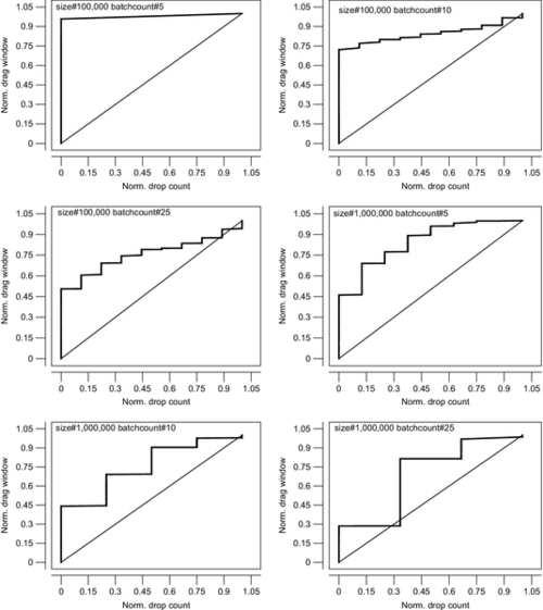
The 6 plots in Fig. 15 are, as before, aggregates based on specific selection rules. Each rule is shown in each plot as the values of parameters applied to the selection. In left-to-right and top-down sequences, the values in the selection rules gradually increase, thus, representing aggregates for relatively light dataset/simulation conditions at first, but gradually moving toward heavier and busier systems.
In Fig. 15, the Drag model shows far worse dynamics than the Drop model — the curve would simply jump from the minimum to the maximum value and stay there. In other words, outcomes for the Drag model are mostly around the upper margin, which explains the shape of the curve. On the other hand, the Drop model has values spread smoothly across the range.
As the aggregates move from lighter to heavier conditions, performance of the Drag model grows less extreme, with gradually more and more values in between the lower and higher extremes. In the bottom-right plot, the curve has moved very close to the diagonal line, indicating that the dynamics of the two packing algorithms are somewhat similar.
There is another way to interpret Fig. 15. Since each curve represents outcomes for the various values for parameters outside of the selector, the curve also offers some insight into whether or not the two packing algorithms can be controlled by changing the operating parameter at runtime. Smoother curves would normally represent a smooth response to changing the parameter, while extreme changes — as those in the top-left plot in Fig. 15, are examples of extreme responses.
This also links back to the discussion of hybrid packing methods which control both the drop rate and window size as part of the same algorithm.
10.6 Summary and Future Directions
This chapter extends the core idea of Big Data Replay into the area of massively multicore hardware environments. The term massively multicore in this chapter is distinct from the well-recognized manycore, both in terms of hardware — the cores on the massively multicore hardware do not need to be supported by special hardware, as is the case of GPU-based or other manycore systems, and in terms of the complexity of the processing logic running on top of such architecture. In the manycore field, cores are built at rigid physical units only loosely attached to the hardware of the host machine — for example, as hardware boards plugs into free slots on the otherwise commodity hardware. Such a design makes it possible for a good degree of isolation between what is running on the manycore board and what is running on the OS back on the host’s own hardware. Manycore systems make extensive use of L1 and L2 hardware caching and have intricate software platforms which use both hardware and software components to offer the highest possible performance.
The massively multicore hardware does not need that level of intense hardware and software support. Given that Big Data processing jobs do not require coordination among each other, a simple hardware with hundreds of cores simply stacked on top of each other should work, in theory. In reality, industry today is mostly invested into manycore systems, which is why there is no hardware that fits the aforementioned description of a massively multicore system. However, based on the advantages of the replay method described in this chapter, there is hope that massively multicore hardware will gather more attention, even if its main applications will be limited to Big Data processing.
The replay method is a drastic change from the traditional Hadoop/MapReduce architecture. While the latter is based on the extreme level of network distribution of its various functions, the former avoids networking and favors one-machine operation. This chapter points to literature by other authors which have already raised the one-machine case, promising, like this chapter, a major improvement in performance.
One reason why one-machine operations may be preferred comes from the fact that network distribution is plagued with various performance bottlenecks. Some of them are discussed by the creators in a paper which denotes clear limits to the throughput of Hadoop/MapReduce clusters. Others — for example, network congestion — are not recognized in traditional Hadoop literature but are discussed in detail in this paper.
Discussing and classifying the various performance bottlenecks takes up a large portion of this chapter. The bottlenecks are first formulated simply by their width (throughput, capacity), but then are expended into a 2D space of ability to isolate versus parallel access, and finally optimized using recent advances in technology, specifically by improving the networking part of the system. As a side note, the replay method depends on one-machine operation, but the cluster is still distributed and depends on networking across the multiple nodes in the clusters. The main difference, however, is that the nodes are supposed to be passive in the replay method, while Hadoop/MapReduce supports a complex environment in which jobs are sent to run on storage nodes, referred to as shards.
An interesting revelation was made in the first two (real) datasets. As a general rule, it is assumed that shared memory can handle much more throughput than storage, even when the latter is based on SSD. However, the experiments reveal that shared memory (shmap library) on commodity hardware performs poorly under a heavy parallel load. In fact, by the definition of the batch-based replay in the chapter, parallel access to shared memory is supposed to be many times heavier than access to storage, which means that the dataset indicates a problem which can be considered normal in such environments.
Performance analysis in this chapter was based on three datasets. The first two came from real-life experiments in the area of parallel access to storage and shared memory, with each experiment run separately. The third dataset was completely synthetic and was used to generate heterogeneous loads based on hotspots. Given the nature of hotspot distribution, the load was extremely heterogeneous. Note that the heterogeneity of jobs is a major concern in recent literature, both in the area of Big Data processing and in multicore parallel programming.
Simulation results show that, even considering performance bottlenecks found in storage and shared memory, the bottleneck of per-item overhead is the narrowest of all, even when distribution of per-item overhead is designed using the hotspot model and the largest hotspots are only allowed to incur, at most, 10 μs overheads. It is unlikely that a real load can offer milder distributions, which means that the throughput restricted by the per-item bottleneck is probably the maximum achievable throughput in objective reality. However, given that many batches and many jobs can run in parallel, the scale of the replay process can alleviate the negative effect of this hard performance bottleneck.
Note that this last revelation calls for comparisons with Hadoop. On one hand, Hadoop is also limited by the per-item bottleneck, which it improves by using network distribution. However, the key difference here is network distribution itself, as the key difference between the two systems. The simple statement offered by this chapter is that scaling inside a single machine is more efficient than scaling over the network. This performance margin is the key difference between Hadoop and the Replay environments.
This research opens upseveral topics for discussion, many of which were addressed in this chapter. The immediately obvious place for improvement is the weakness of shmap in the face of heavy parallel loads. Note that shmap in this chapter was used in the lockfree manner, ie, without locks and with messages that are passive across processes. This means that the overhead found in experiments is solely due to the in-kernel handling of shared memory. There is obviously room for improvement here, without resorting to hardware assistance.
Other venues include the various packing algorithms on top of the two simple ones presented and analyzed in this chapter. Simulation results show that the methods offer some level of flexibility when responding to simulation parameters. This means that a hybrid method which would regulate the drop rate together with window size at runtime could result in better performance than either of the algorithms discussed in this chapter. Moreover, there is a wide range of other parameters that can support alternative methods without resorting to the drop and drag functions. For example, algorithms which remap jobs to other batches rather than drop them entirely might result in a better overall performance of a Replay engine.
Finally, since the single replay node in a cluster is the obvious SPOF, research into running multiple replay nodes in parallel is expected. The main difference with Hadoop here is that replay nodes allow for independent operation and do not depend on syncing across the multiple nodes. Running multiple name nodes in Hadoop, on the other hand, suffers from just that problem, which puts the upper limit on the number of name nodes a Hadoop cluster can handle.