Big Data Analytics on a Smart Grid
Mining PMU Data for Event and Anomaly Detection
S. Wallace; X. Zhao; D. Nguyen; K.-T. Lu
Abstract
Phasor measurement units (PMUs) provide great potential for monitoring an electrical grid by recording synchronized measurements across a wide area. However, with more and more PMUs being deployed, the traditional workflow of processing these data is facing a major challenge. In this chapter, we present our experience in analyzing and mining PMU data for event classification and anomaly detection. Experiments have been carried out using real PMU data that are collected from the Bonneville Power Administration’s power grid. Experimental results show that our methods are effective in identifying both anomalies and known events from a large amount of data. Particularly, our classification method can accurately detect an event from a PMU that is far from the location where the event occurs.
Keywords
Big Data; Smart Grid; Synchrophasors; Phasor measurement unit; Machine learning; Event detection; Anomaly detection
Acknowledgments
The authors would like to thank the Department of Energy/Bonneville Power Administration for their generous support through the Technology Innovation Program (TIP #319) and for providing the PMU data used in this study.
17.1 Introduction
Tomorrow’s Smart Grid will help revolutionize the efficiency of power transmission while also providing improvements in security, robustness, and support for heterogeneous power sources such as wind and solar. The phasor measurement unit (PMU) provides a core piece of technology that measures critical system state variables in a time-coherent fashion across a geographically dispersed area.
PMUs are typically placed at power substations where they generally measure voltage and current phasors (magnitude and phase-angle) for each of the three phases (A, B, and C) as well as frequency and rate of change of frequency. In contrast to legacy systems, PMUs record measurements at high frequency (typically 10–60 Hz [1]) and time stamp each measurement using the global positioning system (GPS). Together, high measurement and precise GPS timestamps create so-called “synchrophasors” or time-synchronized phasors that allow the state of a wide area monitoring system to be observed with high fidelity. Between 2009 and 2014, the number of deployed PMUs within the United States has significantly increased, from ~ 200 PMUs in 2009 [2] to more than 1700 in 2014 [3].
Data from individual PMUs is routed to a phasor data concentrator (PDC) that aggregates and time-aligns the data before passing it on to downstream application consumers. As PMUs and PDCs have become more widely adopted, PDCs have expanded to provide additional data processing and storage functions [4].
Although the comprehensive coverage and high sampling rate of PMUs provide new resources for improving grid operation and control, the data generated by these devices also presents real computational and storage challenges [5]. A typical PMU can measure 16 phasors with a 32-bit magnitude and 32-bit phase-angle. Secondary values such as frequency and rate of change of frequency are also stored as 32-bit values. These, along with 8 bytes for the timestamp and 2 bytes for a PMU operating status flag represent a minimal archival signal set for each device. Recording 60 samples per second, this leads to 5,184,000 samples per day, or ~ 721 MB of data per PMU, per day. However, often there is value in keeping much more data. For example, the Bonneville Power Administration (BPA), who supplies our dataset, has an installed PMU base in the Pacific Northwest of the United States containing roughly 44 PMUs at the time our dataset was collected (2012–14). This dataset requires roughly 1 TB of storage per month of data acquired. Scaling this to the national level then would require more storage by roughly a factor of 40 to incorporate data from all 1700 PMUs.
Traditional approaches for data processing and evaluation are pushed well beyond their feasible limits given the size of the dataset described herein. In this chapter, we describe how cloud computing and methods borrowed from data analytics and machine learning can help transform Smart Grid data into usable knowledge.
17.2 Smart Grid With PMUs and PDCs
Data aggregated by a PDC is sent to downstream consumers in a format defined by IEEE Std. C37.118.2 [1]. The specification indicates two message types that are critical for data analysis: the configuration frame and the data frame.
A configuration frame specifies the number of PMU measurements that are aggregated by the PDC along with the name of the PMU station and the name and type of each signal measured by the station.
A data frame contains the measurements themselves, which have been time-aligned across all stations. Records are fixed-length with no delimiters, and measurements appear in an order prescribed by the configuration frame. Thus, the data frame (with the exception of a short header) can be viewed as a matrix of binary data in which PMU signals span the columns and time spans the rows.
Since this format is readily machine readable, it can also serve as an archival file format. Indeed, the Bonneville Power Administration currently stores archival PMU data as a binary file consisting of: (1) brief metadata including the file specification version; (2) the “active” configuration frame and (3) a data frame typically spanning 60 s of data. This format has the benefit of being entirely self-contained (since a configuration frame is stored along with the data frame); easily portable (1 min of data from roughly 40 PMUs requires about 30 MB of storage) and easily indexed as the flow of time presents a natural mechanism to partition data (eg, by month) using only the filesystem for organization.
17.3 Improving Traditional Workflow
A traditional workflow involving the archival PMU/PDC data may unfold along the following lines:
1. A researcher is notified of an interesting phenomenon at some point in recent history.
2. The researcher obtains archival data for a span of several minutes based on the approximate time of the phenomena.
3. The researcher plots or otherwise analyzes the signal streams over the retrieved timespan to isolate the time and signal locations at which the phenomena are most readily observed.
4. The researcher finally creates plots and performs an analysis over a very specific time range and narrow set of PMU signals as appropriate for the task at hand.
While this workflow is entirely reasonable, it likely leaves the bulk of the data unanalyzed. We view this as a good opportunity to leverage the methods of Big Data analytics and machine learning to turn the latent information in this archived data into useful knowledge.
Specifically, we see the following opportunities:
• characterizing normal operation,
• identifying unusual phenomena, and
• identifying known events.
These operations can all be performed on the historic archive of PMU data using Hadoop/Spark. Typically this would be done at the data center housing that content. Once normal operation has been appropriately characterized, and identification has been performed on the historic data, identification of unusual phenomena and known events can proceed on the incoming (live) PMU data stream in real time with minimal hardware requirements.
17.4 Characterizing Normal Operation
The vast majority of the time, the grid operates within a relatively narrow range of conditions. Many parameters are specified by regulating agencies, and deviation outside of normal conditions may require reporting. As a result, existing infrastructure is well tailored to monitoring for such events. However, smaller deviations in operating conditions that fall below the threshold for reporting are also potentially of interest, both to researchers and operating teams alike. Thus, the first step in identifying such deviations is to characterize normal operation.
A baseline approach for characterizing normal operation is to collect signal statistics across all PMUs. In our work, we began measuring “voltage deviation,” a metric described in [6] and useful for identifying faults (eg, caused by lightning strikes or falling trees).
Voltage deviation is defined as follows:
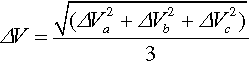
where  and Va represents the voltage of phase A at the point of interest, while ssa represents the steady state voltage of phase A. Thus, voltage deviation represents the three-phase momentary drift away from steady state values.
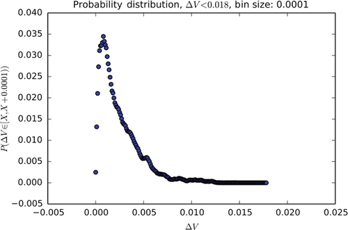
Examining normal operation across 800 min spread across 11 months of BPA’s 2012–13 data yields the histogram shown in Figs. 1 and 2.1 In Fig. 1, we have plotted only bins where the deviation is less than or equal to 0.018 kV. As expected, we see the bulk of the probability mass with very low deviations, and the likelihood of a higher deviation from steady state drops off rapidly from its peak around 0.0007 kV. Plotting the remainder of the observed distribution (ie,  ), one would expect a long tail with a continued slow decay toward zero.
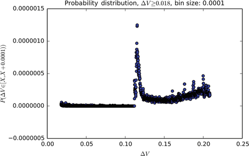
Surprisingly, the distribution shows a secondary spike near 0.12 kV with a noisy decay profile as illustrated in Fig. 2. Note that the y-axis has been scaled for clarity.
By comparing each PMU’s contribution toward the global distribution illustrated herein, we can identify sites that exhibit long-term anomalous behavior. In this case, there is one site contributing to the unusual spike observed above ΔV = 0.10 kV. Removing this site’s contribution from the global histogram results in no observable differences in the shape for values ΔV ≤ 0.018 and a tail that decays more rapidly and smoothly for values of ΔV ≥ 0.018. Further analysis revealed that the unusual tail resulted from data within a few months’ time at the beginning of the data set’s coverage period, signaling a potentially defective or misconfigured device.
17.5 Identifying Unusual Phenomena
Outlier, or anomaly detection, aims to identify unusual examples, in our case, of grid performance. A host of methods exist for this task, some of which are reviewed in Section 17.7. In this chapter, we examine how even the simplest approach, based on the observed probability distribution for normal data, can also be used to find individual moments in time where the data stream is extremely unusual.
Taking the histogram described and illustrated in Section 17.4, we can create a cumulative probability distribution that represents the likelihood that a signal experiences a voltage deviation at or below a given threshold. This operation processes a set of 770 signals from a single day in 16.9 min when performed on our small Spark cluster (4 nodes, 5 GB RAM per node). Once the distribution function has been produced, new data captured from the grid or archived data streamed from disk can be scanned in time, linear, with respect to the number of signals being inspected. Given a distribution function represented as a 1 million element list, we can issue more than 1 million queries per second on commodity hardware using a single core through direct hashing with Python. For our dataset, a 1 million element distribution function has a resolution of 1 V or less. This performance profile well exceeds the requirements for real-time operation.
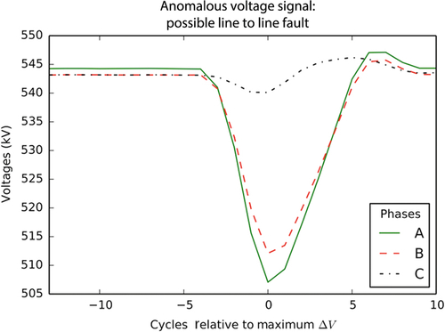
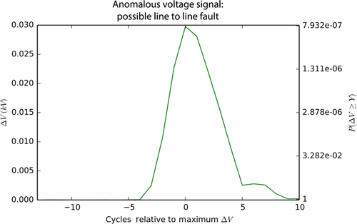
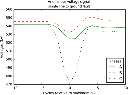
Fig. 3 shows an unusual voltage signature; the corresponding voltage deviation is illustrated in Fig. 4. Note that the scale on the left y-axis of Fig. 4 shows the deviation from steady state while the scale on the right y-axis shows the expected likelihood of the observed deviation based on the histogram data collected previously.2 Although this time period has not been marked by BPA as a line event, the signature is typical of a LL fault, and could represent a fault observed from a distance (perhaps off of BPA’s network). Note that the voltage deviations are low likelihood and the point of maximum deviation has an expected likelihood of less than 7E-7.
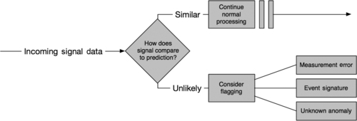
This outlier detection approach can be viewed abstractly as a process of first predicting the next signal value, and then comparing the observed true value to the prediction. A high discrepancy may suggest an event worthy of investigation. The process is illustrated in Fig. 5.
An unlikely observation, such as the ones illustrated in Fig. 3, may be further investigated to determine if they are possible measurement errors, (known) event signatures, or unknown anomalies. Since the grid is a connected system, a change in state variables at one location will impact state variables at other locations. A drop in voltage, as one that occurs with a fault, can be observed across a wide geographical area, although with attenuation based on the electrical distance between sites. A measurement error, then, can be identified as an anomaly that is detected by a single PMU or on a single data stream. Other anomalies (known events or otherwise) will be identified because they create outliers at multiple locations. In the following section, we describe how to further characterize an anomaly observed at multiple sites.
17.6 Identifying Known Events
In contrast to anomaly detection that aims to identify unusual activity using only information about typical (or normal) operational conditions, classification aims to distinguish one type of known event from another. Between 2013 and 2015, we worked with a domain expert to develop a set of hand-coded rules that distinguish between several types of “line faults” that frequently occur on a transmission system: single line to ground (SLG), line to line (LL), and three phase faults (3P) [6,7]. Concurrently, we developed a set of classifiers using machine learning to identify these same fault types. A full comparison of the approaches can be found in [7]. In this chapter, we focus on one specific classifier and discuss performance on both the training and testing data.
We began with a set of events obtained from the Bonneville Power Administration covering an 11 month span between 2012 and 2013. The event dataset includes the time and location of all known line events that occurred on transmission lines that were instrumented with a PMU on at least one end of the line. BPA verified the accuracy of this list and was able to further verify the specific type of event in the majority of cases (60 faults total).
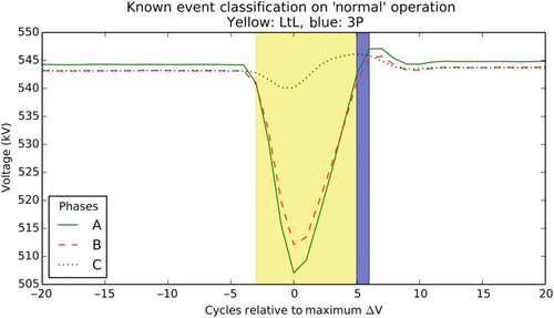
A typical fault is illustrated in Fig. 6. During the event, one or more voltage phases sags and then typically recovers back to steady state voltage within ~ 0.1 s (6 cycles at 60 Hz). Training examples are selected by finding the moment in time where the voltage sags furthest below its steady state value, and then drawing samples from all PMUs (and all voltage phases) at that moment in time. In Fig. 6, this moment occurs at x = 0 cycles (since the x-axis has been labeled relative to the maximum deviation cycle). Thus, this classification process views the data as individual instances, and does not leverage the time-series nature of the data. Note that while we take fault samples at the moment in time where the sag is most extreme, the voltage’s actual deviation from steady state is very much a function of the distance between the PMU making the measurement and the location of the fault itself [8]. Since we take training examples from each PMU for each fault, the actual voltage sags used for training cover a large range of deviations and a fault may be effectively “unobservable” from a PMU that is located far enough from the origin.
Our training set consists of 57 of the 60 faults described herein along with additional samples of normal operation. Three of the original 60 faults were unusable for training because our feature extraction algorithms were unable to process those events (eg, because a specific PMU signal was unavailable at that moment in time). For each fault, we sampled voltage from all available PMUs. In total, this method yields 4533 data points, of which 4135 are SLG faults, 348 are LL faults, and 50 are 3P faults. To this set, we add 17,662 data points sampled from roughly 800 min of normal operation over the one-year period. We randomly selected half (8831) of these normal samples to use for training. In all, this represents 12,966 training samples of both normal operation and fault condition.
Fig. 7 shows the performance of the decision tree that is inferred using the training data described herein. The figure shows two matrices: the matrix on the left indicates Boolean fault-detection performance while the matrix on the right indicates refined classification into the three fault types (SLG, LL, and 3P) and the “Normal” class. Each cell contains two values. The value at the top represents the prediction at the PMU nearest to the fault (there are 57 of these, one for each fault in the training set). The value at the bottom of each cell represents the predicted class for all measurements that occur at PMUs further from the fault. Note that for “Normal” data, there is no notion of a fault location, and thus the top value in the rows labeled “Normal” is always zero.
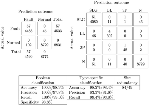
The table following the matrices illustrates performance characteristics on the training data. For most measurements, we include the measurement at the fault location and across the grid as a whole (on the left and right side of the slash, respectively). In the table, site redundancy indicates the number of PMU signals (ie, the number of voltage signals) that detect each fault where the value on the left of the slash is the median redundancy and the number on the right represents the fifth percentile redundancy. For these results, a fifth percentile redundancy of 49 indicates that 95% of the faults are detected by 49 different voltage measurements in the dataset (where one voltage measurement includes all three phases: A, B, and C). Note that each PMU often makes multiple voltage measurements for different substation buses, and at times, for individual transmission lines as well. So for our dataset, this number tends to be larger than the number of actual PMUs.
Fig. 8 illustrates the performance of the same decision tree on a test set that was unseen during training. Test data here was obtained using the same procedure outlined in [7]. That is, test instances are obtained for faults from the moment prior to the largest voltage deviation (cycle − 1 in Fig. 6). This approach yields the same number of test instances as training instances and in some sense is a more challenging test than randomly partitioning the training and testing set because this method guarantees that test instances will have an equal or smaller deviation from steady state as compared to training instances. For simplicity of comparison, we show the performance relative to the training set. Note that at the fault location, there are no changes to the classification results. As we consider PMUs further afield, however, we acquire more errors than with the training set.
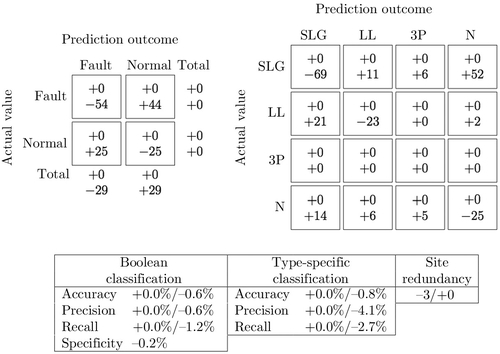
Fig. 9 illustrates the performance of the decision tree when applied to the data in the vicinity of the anomaly from Figs. 3 and 4. Viewed by itself, the classifier does a good job of identifying the main voltage signature (the drop below steady state that occurs between cycles − 2 and 5) as a probable LL fault. However, it makes a poor prediction at cycle 5, where the voltage has almost returned to steady state values. Here, the classifier predicts a 3P. Note that if we combine the predictions with the likelihood information in Fig. 4, it is easy to constrain the event predictor to only those signals that are relatively unlikely to occur in normal operation. For example, if we set the likelihood threshold at 1E-6, then only the predictions at x = − 1 … 1 will be created. Not coincidently, this is when the classifier also gives the best predications.
17.7 Related Efforts
Smart grid technology provides great potential to build more reliable electrical grid systems by utilizing advanced digital and communication technologies. However, with the worldwide initiative of upgrading the traditional electrical grid to the Smart Grid, new challenges have been introduced, among which is the “Big Data” challenge. The Smart Grid generates a significant amount of data on a daily basis, and these data must be processed in an efficient way in order to monitor the operational status of the grid. As machine learning techniques have become the de facto approaches for Big Data analytics, these techniques are also applied and adapted to process and analyze PMU data. A common objective of the PMU data analysis is to recognize and identify patterns, or signatures of events that occur on the Smart Grid. Therefore, a large number of these approaches are based on pattern recognition [9].
For identifying signatures of known events, classification approaches, or detection trees, are proven to be most effective. For instance, in [10], a classification method is proposed for tracing the locations where faults occur on a power grid. This method is based on the pattern classification technology and linear discrimination principle. Two features of the PMU data are used in the classification: nodal voltage, and negative sequence voltage. For localizing a fault, irrelevant data elements are identified and filtered out using linear discriminant analysis. Similar classification technologies can also be used to identify other signatures of events in power systems, such as voltage collapse [11] and disturbances [12]. Diao et al. [11] develop and train a decision tree using PMU data to assess voltage stability. The decision tree is threshold based, and it can be used to evaluate both static and dynamic post-contingency power system security. A J48 decision tree is used in [7] for classifying different types of line faults using a set of novel features derived from voltage deviations of PMU data, and this approach greatly improves the accuracy of detecting line faults from a distance, compared with an approach based on an expert’s hand-built classification rules. In Ray et al. [12] build support vector machines (SVMs) and decision tree classifiers based on a set of optimal features selected using a genetic algorithm, for the purpose of detecting disturbances on the power grid. SVM-based classifiers can also be used to identify fault locations [13], and predict post-fault transient stability [14].
For anomaly detection, machine learning techniques are often applied for detecting security threats, such as data injections or intrusions, instead of detecting bad data measurements. The latter is usually addressed by developing PMU placement algorithms that allow measurement redundancy [15,16]. In [17], various machine learning methods are evaluated to differentiate cyber-attacks from disturbances. These methods include OneR, Naive Bayes, SVM, JRipper, and Adaboost. Among these approaches, the results show that applying both JRipper and Adaboost over a three-class space (attack, natural disturbance, and no event) is the most effective approach with the highest accuracy. Pan et al. [18] propose a hybrid intrusion system based on common path mining. This approach aggregates both synchrophasor measurement data and audit logs. In addition, SVMs have also been used in detection data cyber-attacks. For instance, Landford et al. [19] proposes a SVM based approach for detecting PMU data spoofs by learning correlations of data collected by PMUs which are electrically close to each other.
Due to the time sensitivity of event and anomaly detection on the Smart Grid, a major challenge of applying machine learning techniques to perform these tasks is the efficiency of these approaches. This is especially important for online detection of events. Two different types of approaches have been used to address this challenge. Dimensionality reduction [20] is a commonly used approach to improve learning efficiency by reducing the complexity of the data while preserving the most variance of the original data. A significant amount of efforts have been made in this direction. For instance, Xie et al. [21] propose a dimensionality reduction method based on principal component analysis for online PMU data processing. It has been shown that this method can efficiently detect events at an early stage. In [22], a similar technique is used to reduce the dimensionality of synchrophasor data by extracting correlations of the data, and presenting it with their principal components. Another type of approach for improving the efficiency of PMU data processing is to adopt advanced high-performance computing and cloud computing techniques, such as Hadoop [23], and the data cloud [24].
Although a variety of machine learning techniques have been proposed to analyze PMU data for event classification and anomaly detection, very few have been applied to real PMU data collected from a large-scale wide area measurement system (WAMS). Gomez et al. [14] apply a SVM based algorithm to a model of practical power system. However, the number of PMUs considered is restricted to 15. Most other approaches are based on simulations. The work presented in this chapter, in contrast, is based on mining real PMU data collected from BPA’s transmission grid.
17.8 Conclusion and Future Directions
We presented our experience in mining PMU data collected from BPA’s WAMS, for the purpose of detecting line events, and anomalies. This work aims for improving the traditional workflow of analyzing archival PMU data to identify events. Specifically, we first characterize the PMU data collected during the period when the grid is under normal operational status. Based on the statistical results obtained in this step, we can easily identify outliers by examining the likelihood of the measurement indicated by the probability distribution of the normal data. Besides anomaly detection, we have also developed a classification method using machine learning techniques for identifying known events, namely SLG, LL, and 3P. The experimental results on our dataset show that our classification method can achieve high accuracy in detecting these events, even when the PMU site is far away from the fault location.
Work is ongoing in several directions. First, we are examining other learning algorithms for event classification. To this end, instead of using an existing classification algorithm, we are building our own decision tree by leveraging other machine learning techniques, such as SVMs. Second, we are also applying unsupervised clustering techniques to PMU data. Different from the classification approach in which sufficient labeled data are needed for training purposes, clustering approaches do not require substantial labeled data. This approach can potentially identify unknown events and signatures similar to anomaly detection, but with the added benefit of identifying potential relationships between anomalies. Third, we are repurposing these machine learning techniques to solve different problems in the power grid domain, eg, data cleansing and spoofed signal detection. Finally, building on our understanding of the Smart Grid, we are investigating novel interaction models and resource management approaches to support energy-efficient data centers powered by the Smart Grid.