Chapter 5

Integrators and Planimeters

To describe the next major advance in the field of computing and to set the stage for our real topic, the early history of the electronic digital computer, we need to embark on an excursus. It is desirable at this point to acquaint those of our readers who are not already familiar with them with the differences between digital and analog or continuous computing instruments. These are the two broad categories into which we can divide all forms of computing equipment or processes.

Every computing instrument or machine of whatever sort has certain fundamental operations which it performs and out of which are formed its overall operations. Thus Pascal’s machine had addition and subtraction as its operations; Leibniz’s had addition, subtraction, multiplication, and division as its; Babbage’s Difference Engine had addition and subtraction.

In these three cases the fundamental operations were performed by the well-known techniques of counting, that is, they did their fundamental operations by a mechanization of the methods that we as humans employ. Machines of this class are generically described as digital or arithmetical. The former name clearly calls attention to the quantities employed and the latter to the processes performed on these quantities. The premier device in this category is the abacus, the simplest form of digital computer still used in many places throughout the world.

Analog machines are very different. They are often described as being continuous or measurement. They are rather difficult to explain and describe. Here the former name again calls attention to the quantities employed and the latter to the processes performed on them. In all cases analog machines depend upon the representation of numbers as physical quantities such as lengths of rods, direct current voltages, etc. Usually they are developed for a fairly specific purpose.

During the latter part of the nineteenth century physicists had developed sufficient mathematical sophistication to describe in mathematical equations the operation of fairly complex mechanisms. They were also able to perform the converse operation: Given a set of equations, to conceive a machine or apparatus whose motion is in accord with those equations.1 This is why these machines are called analog. The designer of an analog device decides what operations he wishes to perform and then seeks a physical apparatus whose laws of operation are analogous to those he wishes to carry out. He next builds the apparatus and solves his problem by measuring the physical, and hence continuous, quantities involved in the apparatus. A good example of an analog device is the slide rule. As is well-known, the slide rule consists of two sticks graduated according to the logarithms of the numbers, and permitted to slide relative to each other. Numbers are represented as lengths of the sticks and the physical operation that can be performed is the addition of two lengths. But it is well-known that the logarithm of a product of two numbers is the sum of the logarithms of the numbers. Thus the slide rule by forming the sum of two lengths can be used to perform multiplication and certain related operations.

Another old but important analog device is the planimeter, a device for measuring the area bounded by a simply closed curve (Fig. 1).

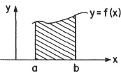
Fig .1

George Stibitz in an article on mathematical instruments attributes the first such device to a German engineer, J. H. Hermann, in 1814.² In any case various improved versions appeared both on the Continent and in Britain. The most famous names connected with these are James Clerk Maxwell, who invented one in 1855, and James Thomson (1822–1892), who produced one in the early 1860s based on Maxwell’s. Thomson presented his idea to the Royal Society in 1876. The delay was occasioned by the fact that Thomson saw no use for the instrument until his brother, Lord Kelvin, discussed with him an idea for a tide-calculating machine. At that point it became clear that his integrator could provide exactly what was needed. Thomson wrote thus: “The idea of using pure rolling instead of combined rolling and slipping was communicated to me by Prof. Maxwell, when I had the pleasure of learning from himself some particulars as to the nature of his contrivance…. I succeeded in devising for the desired object a new kinematic method…. Now, within the last few days, this principle, on being suggested to my brother as perhaps capable of being usefully employed towards the development of tide-calculating machines which he had been devising, has been found by him to be capable of being introduced and combined in several ways to produce important results.”3

In all these analog devices the fundamental operation is that of integration, i.e. they all produce as an output given f(x) as an input. (The reader will recall this is the same as the area marked in by slanted lines in Fig. 1 above.)

If one were asked to name the great British physicists of the nineteenth century, or indeed of all time, James Clerk Maxwell’s name would very likely be next to that of Newton’s. It is not our place here to describe either his life or work but we must at least indicate his most famous and wonderful accomplishment: a complete treatment of the relation between light and electromagnetism, by means of a mathematical theory resting on two fundamental equations. His work is basic to all our understanding of electricity, magnetism, light, and other forms of electromagnetic radiation. In his monumental work, A Treatise on Electricity and Magnetism, he not only expressed in his equations the beautiful experimental findings of Michael Faraday (1791–1867) but also predicted the existence of electromagnetic waves, which we will discuss briefly later.

For the benefit of those readers who do not know how integrators and planimeters work, we quote Maxwell’s own description since it so well describes the situation:

In considering the principle of instruments of this kind, it will be most convenient to suppose the area of the figure measured by an imaginary straight line, which, by moving parallel to itself, and at the same time altering in length to suit the form of the area, accurately sweeps it out.

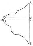
Let AZ be a fixed vertical line, APQZ the boundary of the area, and let a variable horizontal line move parallel to itself from A to Z, so as to have its extremities, P and M, in the curve and in the fixed straight line. Now, suppose the horizontal line (which we shall call the generating line) to move from the position PM to QN, MN being some small quantity, say one inch for distinctness. During this movement, the generating line will have swept out the narrow strip of the surface, PMNQ, which exceeds the portion PMNp by the small triangle PQp.

But since MN, the breadth of the strip, is one inch, the strip will contain as many square inches as PM is inches long; so that, when the generating line descends one inch, it sweeps out a number of square inches equal to the number of linear inches in its length.

Therefore, if we have a machine with an index of any kind, which, while the generating line moves one inch downwards, moves forward as many degrees as the generating line is inches long, and if the generating line be alternately moved an inch and altered in length, the index will mark the number of square inches swept over during the whole operation. By the ordinary method of limits, it may be shown that, if these changes be made continuous instead of sudden, the index will still measure the area of the curve traced by the extremity of the generating line.

. . . . . . . . . . . . . . . . . . . . . . . . . . . . . . . . . . . . . . . . . . . . . .

We have next to consider the various methods of communicating the required motion to the index. The first is by means of two discs, the first having a flat horizontal rough surface, turning on a vertical axis, OQ, and the second vertical, with its circumference resting on the flat surface of the first at P, so as to be driven round by the motion of the first disc. The velocity of the second disc will depend on OP, the distance of the point of contact from the centre of the first disc; so that if OP be made always equal to the generating line, the conditions of the instrument will be fulfilled.

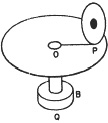
This is accomplished by causing the index-disc to slip along the radius of the horizontal disc; so that in working the instrument, the motion of the index-disc is compounded of a rolling motion due to the rotation of the first disc, and a slipping motion due to the variation of the generating line.4

It remained for Lord Kelvin—then Sir William Thomson—to make fundamental use of integrators to build some machines which could really do work transcending what a human could. Kelvin in his long life was enormously broad in his interests and worked in virtually every aspect of the physics of his day. One subject seemed to have great attraction for him: the motion of the tides. To gain an understanding of tidal motion, he invented several instruments which played an important part in this task. They are a tide gauge, a tidal harmonic analyser, and a tide predictor.⁵

The first of these instruments does not concern us except in a passing way. It is intended to record “by a curve traced on paper, the height of the sea level at every instant above or below some assumed datum line.” The second is much more germane to our discussion. Kelvin, writing about his tidal harmonic analyser, said: “The object of this machine is to substitute brass for brain in the great mechanical labour of calculating the elementary constituents of the whole tidal rise and fall…. The machine consists of an application of Professor James Thomson’s Disk-Globe-and-Cylinder Integrator to the evaluation of the integrals required for the harmonic analysis…. It remains now to describe and explain the actual machine … which is the only Tidal Harmonic Analyser hitherto made.”6

Let us now turn attention to a few of the details of his harmonic analyser and tide predictor. To do this it is convenient first to discuss very briefly what is meant by simple harmonic motion.

Perhaps the easiest example of simple harmonic motion is afforded by musical instruments and in particular by musical notes, as distinguished from noise. Such notes correspond to periodic vibrations, i.e. after a certain interval of time, called the period, those vibrations repeat themselves with perfect regularity. The number of vibrations made in a given time is referred to as the frequency. Finally, the notes whose frequencies are multiples of that of a given one, are called its harmonics.

However, musical notes, while periodic, are frequently made up of simpler vibrations called tones or simple harmonic motions. It has been shown that these tones are mathematically representable by the so-called circular functions, the sines and cosines of trigonometry. What are these functions or simple motions? Let us imagine a point P which is moving uniformly—at constant speed—around a circle and let us drop a perpendicular from this point P to the diameter as in Fig. 2 below. The perpendicular cuts the diameter at a point Q which moves back and forth along the diameter. The motion of Q is what is called simple harmonic motion.

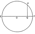
Fig .2

Before going into more details we should remark that the reader who finds mathematical formulas unfamiliar or even frightening can safely skip over these in the text. They are introduced for possibly pedantic reasons by the author and may be safely ignored.

Now in Fig. 3 the amplitude of the motion is the distance r = OE = OF; the period is the time it takes Q to go from its present position—whatever that may be—back to the same position and moving in the same direction as it was. This is represented mathematically as

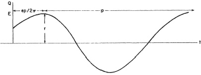
Fig .3

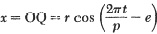
where r is the radius of the circle or the amplitude, p is the period, t is the time, and e is the phase or phase angle. This phase measures essentially when we start reckoning time, i.e., at t = ep/2π we have x = r. Different simple harmonic motions may, or course, start at different times. They are thus out of phase with each other.

These simple facts about musical tones or simple harmonic motion apply equally to all types of periodic motions. Such motions are particularly important in physics since very many phenomena are periodic—indeed, our lives are constantly regulated by such motions, as for example the rotation of the earth about its axis on a daily basis or its revolution about the sun on a yearly one. Many such examples can be cited, but that is not the point. The study of simple harmonic motions probably sounds to the uninformed reader as possibly interesting but certainly highly special.

That this is not the case was first shown by a most remarkable man, Jean-Baptiste-Joseph Fourier (1768–1830), the orphaned son of a tailor in Auxerre, France. According to Bell:

By the age of twelve he was writing magnificent sermons for the leading church dignitaries of Paris to palm off as their own. At thirteen he was a problem child, wayward, petulant, and full of the devil generally. Then, at his first encounter with mathematics, he changed as if by magic. He knew what ailed him and cured himself. To provide light for his mathematical studies after he was supposed to be asleep he collected candle-ends in the kitchen and wherever he could find them in the college. His secret study was an inglenook behind a screen….

To check the mere blood-letting Napoleon ordered or encouraged the creation of schools. But there were no teachers. All the brains that might have been pressed into immediate service had long since fallen into the buckets. It became imperative to train a new teaching corps of fifteen hundred, and for this purpose the École Normale was created in 1794. As a reward for his recruiting in Auxerre Fourier was called to the chair of mathematics.7

In 1807 he wrote a treatise on the mathematical theory of heat, Théorie analytique de la chaleur, that is now world famous. In it is contained a theorem, now named after him, which is described by Thomson and Tait as follows: “Fourier’s theorem … is not only one of the most beautiful results of modern analysis, but may be said to furnish an indispensable instrument in the treatment of nearly every recondite question in modern physics.”⁸

This result may be described roughly in this way: An extremely wide class of periodic phenomena are describable as a sum of a simple harmonic motion and of its harmonics with suitably chosen amplitudes. Thus the physicist may resolve virtually any complex periodic vibration or motion into simple ones based on the familiar sines and cosines of trigonometry. In mathematical language we may write a periodic function/as

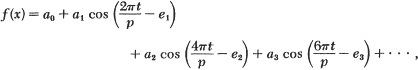
where the number of terms in the sum may be finite or infinite. If we permit not only cosines but also sines, the phase angles may be eliminated, and we write

Even the case where there are only two periodic terms in the series can be quite interesting. If one considers the lunar and solar tides, they are each found to be very nearly simple harmonic motions—except in certain cases such as tidal rivers or long channels or deep bays. Thus in many cases one can as a first approximation consider tidal motion as the sum of just these two simple harmonic ones. (The amplitude of the lunar tide is about twice that of the solar one.) The interested reader is referred to Thomson and Tait for the details.

We are now in a much better position to describe what a harmonic analysis is and how a harmonic analyser does it. First of all, given a periodic function or phenomenon, then a harmonic analysis of it is a determination of the amplitudes of the fundamental and its overtones or harmonics. That is, a harmonic analysis of a given periodic phenomenon is intended to find the coefficients b₀, b₁ etc. and c₁ c₂, etc. in our formula for f(x).

It may be shown by the mathematically inclined reader that the coefficients are expressible as

Thus a harmonic analysis consists of forming a number of integrals of the general form

where g is a sine or cosine function. The evaluation of integrals of this sort is what Kelvin succeeded in doing by an ingenious adaptation of his brother’s disk-globe-and-cylinder integrator. In fact he says: “… and I believe that in the application of it to the tidal harmonic analysis he will be able in an hour or two to find by aid of the machine any one of the simple harmonic elements of a result which hitherto has required not less than twenty hours of calculation by skilled arithmeticians.”9 We need not go now into the details of how he carried out the adaptation.

Here we see for the first time an example of a device which can speed up a human process by a very large factor, as Kelvin asserts.

That is why Kelvin’s tidal harmonic analyser was important and Babbage’s difference engine was not.

Maxwell in an aricle on harmonic analysis stated:

Sir W. Thomson, availing himself of the disk, globe, and cylinder integrating machine invented by his brother, Professor James Thomson, has constructed a machine by which eight of the integrals required for the expression of Fourier’s series can be obtained simultaneously from the recorded track of any periodically variable quantity, such as the height of the tide, the temperature of the pressure of the atmosphere, or the intensity of the different components of terrestrial magnetism. If it were not on account of the waste of time, instead of having a curve drawn by the action of the tide, and the curve afterwards acted on by the machine, the time axis of the machine itself might be driven by a clock, and the tide itself might work the second variable of the machine, but this would involve the constant presence of an expensive machine at every tidal station.

It would not be devoid of interest, had we opportunity for it, to trace the analogy between these mathematical and mechanical methods of harmonic analysis and the dynamical processes which go on when a compound ray of light is analyzed into its simple vibrations by a prism, when a particular overtone is selected from a complex tune by a resonator, and when the enormously complicated sound-wave of an orchestra, or even the discordant clamours of a crowd, are interpreted into intelligible music or language by the attentive listener, armed with the harp of three thousand strings, the resonance of which, as it hangs in the gateway of his ear, discriminates the multifold components of the waves of the aerial ocean.10

Another interesting use for a harmonic analyser may be noted. Kelvin also built a small harmonic analyser which could be used to handle the analysis needed to adjust the compasses in iron ships—a process that was still in use in World War II. The instrument was capable of handling harmonic functions of the form

This is precisely the form the deviation of the compass needle from the true reading takes as a function of the heading angle 0 of the ship; once the coefficients A, B, …, E are known small blocks of iron are inserted into the compass housing to compensate for the deviation.

The tide predictor of Kelvin is an interesting and important instrument based on his harmonic analyser. In his words: “After having worked for six years at the Tidal Harmonic Analysis the Author designed an instrument for performing the mechanical work of adding together the heights (positive or negative) above the mean level, due to the several simple harmonic constituents, determined by analysis, from observation or from the curves of a self-recording tide gauge for any particular part, so as to predict for the same port for future years, not merely the tides of high and low water, but the position of the water-level at any instant of any day of the year.”11

The last of Kelvin’s inventions that is relevant to our history at this point is his work on what is now called a differential analyzer. In a most interesting preliminary paper he set himself the task of mechanically integrating the most general linear differential equation of the second order. This is a very important equation to the mathematical physicist because it describes, inter alia, “vibrations of a non-uniform stretched cord, of a hanging chain, of water in a canal of non-uniform breadth and depth, of air in a pipe of nonuniform sectional area, conduction of heat along a bar of nonuniform section or non-uniform conductivity, Laplace’s differential equation of the tides, etc., etc.” It is also of great importance to electrical engineers since many circuits can be described by means of it.

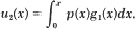
Kelvin put his differential equation into the form

where p is a given function of x. He then set up an iterative scheme whereby he made an initial guess for u, say u₁. He then envisioned a device containing two integrators so that he could form by the first integrator

and then by the second one

He then took his result u₂ and put it into the first integrator in place of u₁ and repeated his procedure, finding u₃, etc. It is known that this procedure will in general converge. In Kelvin’s words: “After thus altering, as it were, u₁ into u₂ by passing it through the machine, then u₂ into u₃, by a second passage through the machine, and so on, the thing will, as it were, become refined into a solution which will be more and more nearly rigorously correct the oftener we pass it through the machine. If u_i+1 does not sensibly differ from u_i, then each is sensibly a solution.”12

This point of view, while interesting, still lacked something which apparently came to Kelvin in 1876. He wrote: “So far I had gone and was satisfied, feeling I had done what I wished to do for many years. But then came a pleasing surprise. Compel agreement between the function fed into the double machine and that given out by it…. Thus I was led to a conclusion which was quite unexpected; and it seems to me very remarkable that the general differential equation of the second order with variable coefficients may be rigorously, continuously, and in a single process solved by a machine.”¹³

To describe exactly what Kelvin meant we need now to pause for a moment. Observe that in Kelvin’s second integral appears the function g₁(x) calculated in the first one. What he now noticed was that if the result of the second integration is continuously fed into the first integral, it forces u = u₁ to be u₂ and in one iteration the problem is solved. In differentials we have

under this scheme. Now if we eliminate g₁ from these relations, we have

In other words, u is the solution of the differential equation.

This technique can of course be generalized, and Kelvin wrote another paper entitled Mechanical Integration of the General Linear Differential Equation of Any Order with Variable Coefficients.¹⁴ This paper contains basically the idea which Vannevar Bush was to rediscover when he developed and constructed the first successful machine to do what Kelvin proposed,

The difficulty with Kelvin’s scheme was technological and he never built a machine for solving differential equations. The problem arises from the need to take out the output of one integrator and use it as the input to another. Why is this a difficulty? The answer lies in the fact that, in Maxwell’s explanation, the output is measured by the rotation of a shaft attached to a wheel that is turned by pressing on a rotating disk. The so-called torque of this shaft—its ability to turn another shaft—is very slight and hence it cannot in fact form the input to another integrator. This was to be a barrier to progress for fifty years.

1 S. Lilley, “Machinery in Mathematics, A Historical Survey of Calculating Machines, ” Discovery, vol. 6 (1945), pp. 150–182. See also, Lilley, “Mathematical Machines, ” Nature, vol. 149 (1942), pp. 462–465.

² Encyclopaedia Britannica (1948), s.v. “mathematical instruments.”

³ Thomson and Tait, Principles of Mechanics and Dynamics, Appendix B’: III, “An integrating Machine having a new Kinematic Principle, ” pp. 488–490.

⁴ The Scientific Papers of James Clerk Maxwell (Dover edition, New York, 1965), pp. 230–232; the paper itself is entitled “Description of a New Fonn of the Plato-meter, an Instrument for Measuring the Areas of Plane Figures drawn on Paper, ” and first appeared in Transactions of the Royal Scottish Society of Arts, vol. IV (1855).

⁵ Kelvin, Mathematical and Physical Papers, vol. VI, pp. 272ff.

⁶ Kelvin, Papers, vol. VI, p. 280.

⁷ Bell, Men of Mathematics, chap. 12.

⁸ Thomson and Tait, op. cit., part 1, p. 54.

⁹ Sir W. Thomson, Proc. Roy. Soc. vol. 24 (1876), p. 266; see also Thomson and Tait, p. 496.

¹⁰ J. C. Maxwell, “Harmonic Analysis, ” Collected Works, H, 797–801.

¹¹ Kelvin, Papers, vol. VI, p. 285.

¹² Thomson and Tait, part 1, p. 498.

¹³ Ibid.

¹⁴ Thomson and Tait, p. 500.