6- Introduction to DAX Measures

“The Best Thing to Happen to Excel in 20 Years”

That’s a quote from Mr. Excel himself, Bill Jelen. He was talking about PowerPivot in general, but specifically measures. So what are measures?

On the surface, you can think of Measures as “formulas that you add to a pivot.” But they offer you unprecedented power and flexibility, and their benefits extend well beyond the first impression. Several years after I started using PowerPivot professionally, I am still discovering new use cases all the time.

Aside: A Tale of Two Formula Engines

Some of you may already be saying, “hey, pivots have always had formulas.”

Why yes, yes they have. Here’s a glimpse of the formula dialog that has been in Excel for a long time:

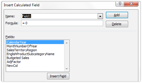
Figure 36 PowerPivot measures mean that you will NEVER use this “historical” pivot formula dialog again (if you ever used it at all)

This old feature has never been all that helpful, nor has it been widely used. (Oh and if you think it has been helpful, great! PowerPivot measures do all of this and much, much more).

It has not been very helpful or widely used because it never received much investment from the Excel team at Microsoft. The Excel pivot formula engine is completely separate from the primary formula engine (the one that is used on worksheets). Whenever it came time for us to plan a new version of Excel, we had to decide where to spend our engineering budget. The choice between investing development budget in features that everyone sees, like the worksheet formula engine, versus investing in a relatively obscure feature like this, was never one which required much debate. The pivot formula engine languished, and never really improved.

Remember the history of PowerPivot though? How I said it sprang from the longstanding SSAS product? Well, SSAS is essentially one big pivot formula engine. So now, all at once, we have a pivot formula engine that is the result of nearly 20 years of continuous development effort by an entire engineering team. Buckle up :-)

Adding Your First Measure

There are two places where you can add a measure:

1. In the Excel window (attached to a pivot)

2. In the PowerPivot window (in the measure grid). Note that this is called Calculation Area in the UI but I call it the measure grid since it only contains measures.

I highly recommend starting out with the first option – in the Excel window, attached to a pivot, because that gives you the right context for validating whether your formula is correct.

Create a Pivot

With that in mind, I use the pivot button on the ribbon in the PowerPivot window.

Figure 37 Creating a pivot

I could also use the similar button on the PowerPivot ribbon tab in the Excel window – they do exactly the same thing. I do NOT recommend using the pivot buttons on the Insert tab of the Excel window however, as that leads to a different experience.

This yields a blank pivot on a new worksheet:

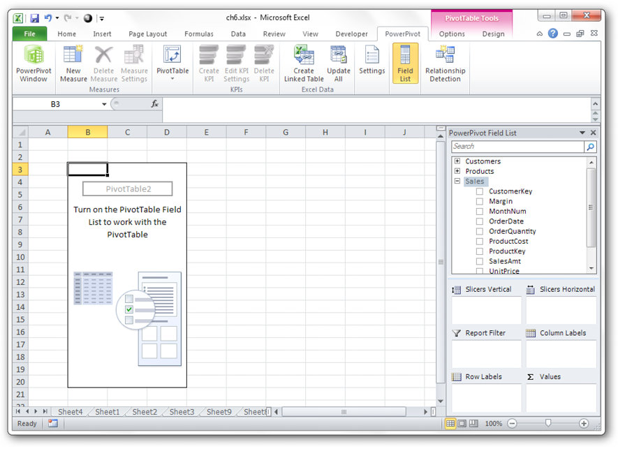
Figure 38 Blank pivot

Notice how the pivot field list contains all three tables from the PowerPivot window?

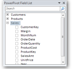
Figure 39 Every table from the PowerPivot window is available in the field list

For now, we are going to ignore the other tables and just focus on Sales. Exploring the advantages of multiple tables is covered later on.

Add a Measure!

I’m going to click the New Measure button on the PowerPivot ribbon tab in Excel:

Figure 40 New Measure Button

This brings up the Measure Settings dialog, which I will often refer to as the measure editor, or often as just “the editor.”

In Excel 2013, “Measures” are no longer called “Measures.” They are now called “Calculated Fields,” taking over the name of the old (and much more limited) feature that I made fun of at the beginning of this chapter. I’m pretty sure I will call them “measures” forever, and I will continue to use that word in this book. In the meantime though, here’s the entry point on the Excel 2013 ribbon.

Figure 41 The equivalent entry point in Excel 2013, where Measures are now called Calculated Fields. This leads to the same editor (below) as the original “New Measure” button in PowerPivot V1 and V2.

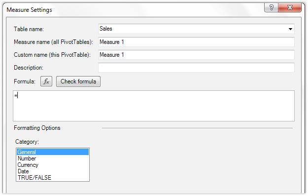
Figure 42 Measure Settings, also known as the Measure Editor, or The Editor :-)

There’s a lot going on in this dialog, but for now let’s ignore most of it and just write a simple formula:

=SUM(Sales[SalesAmt])

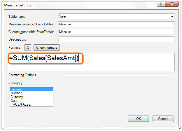
Figure 43 Entering a simple measure formula

Name the Measure

Before clicking OK, I will give the measure a name. This is just as important as giving sensible names to tables and columns.

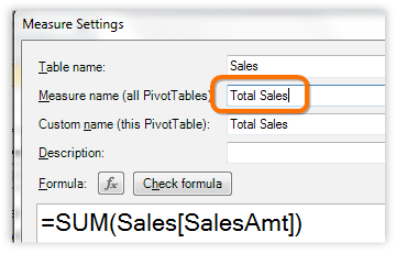
Figure 44 It is very important to give the measure a sensible name

The “Measure name” box is the one you want to fill in. Ignore the “Custom name” box for now – that will automatically match what you enter in the “Measure name” box.

Results

Click OK, and I get:

Figure 45 The resulting pivot

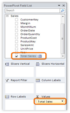
Figure 46 New checkbox added to the field list for the measure, and measure added to Values dropzone

Works As You Would Expect

Let’s do some “normal pivot” stuff. I’ll going to drag MonthNum to Rows and Year to Columns, yielding:

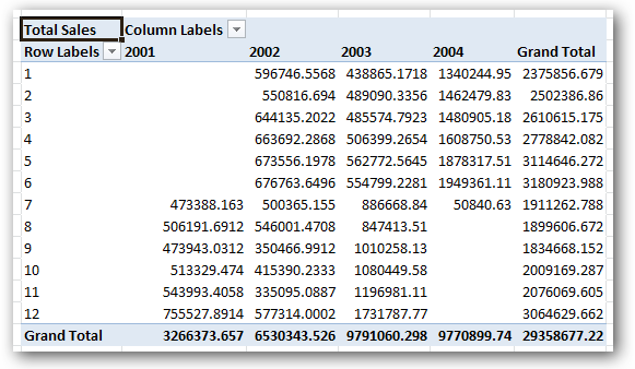
Figure 47 MonthNum field on Rows, Year on Columns, Total Sales Measure just “does the right thing”

OK, our first measure is working well. Let’s take stock of where we stand before moving on.

“Implicit” versus “Explicit” Measures

We have done nothing special so far, we are just laying the groundwork. I mean, a simple SUM of the SalesAmt column is something I always could have done in normal pivots.

In fact, I can uncheck the [Total Sales] measure and then just click the [SalesAmt] checkbox, and get precisely the same results as before:

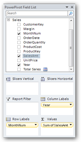
Figure 48 Unchecked the [Total Sales] measure, checked the [SalesAmt] checkbox

Figure 49 Yields the same exact pivot results

Just like in normal pivots, if you check the checkbox for a numerical column, that will default to creating a SUM in the Values area of the field list. And checking a non-numeric field will place that field on Rows by default.

So we have two ways to “write” a SUM in PowerPivot – we can write a formula using the Measure Editor, or we can just check the checkbox for a numeric column.

I have my own terms for this:

1. Explicit Measure – a measure I create by writing a formula in the Editor

2. Implicit Measure – what I get when I just check a numeric column’s checkbox

Turns out, I have a very strong opinion about which of these is better.

I never, ever, EVER create implicit measures! Even if it’s a simple SUM that I want, I always fire up the measure editor, write the formula, and give the measure a sensible name. I think it is important that checking a numeric checkbox does what it does, because that matches people’s expectations from normal Excel. But that does not mean you should do it! Trust me on this one, you want to do things explicitly. There are too many benefits to the explicit approach. You will not see me create another implicit measure in this book. They are dead to me :-)

Referencing Measures in Other Measures

I’ll show you one reason why I prefer explicit measures right now.

Another Simple Measure First

First, let me create another simple SUM measure, for Margin:

=SUM(Sales[Margin])

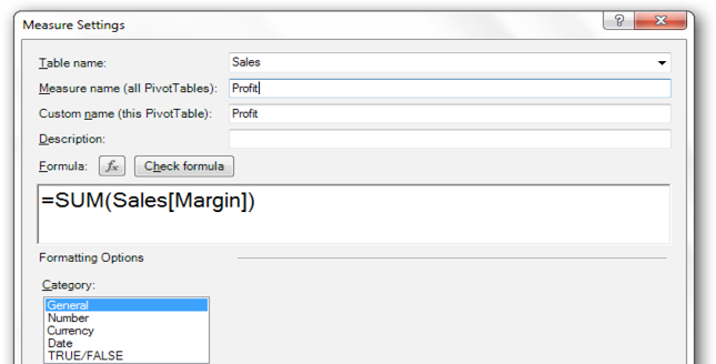
Figure 50 Creating a new measure, that I named Profit

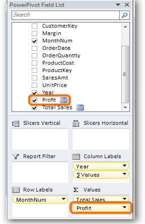
Figure 51 Profit measure added to field list

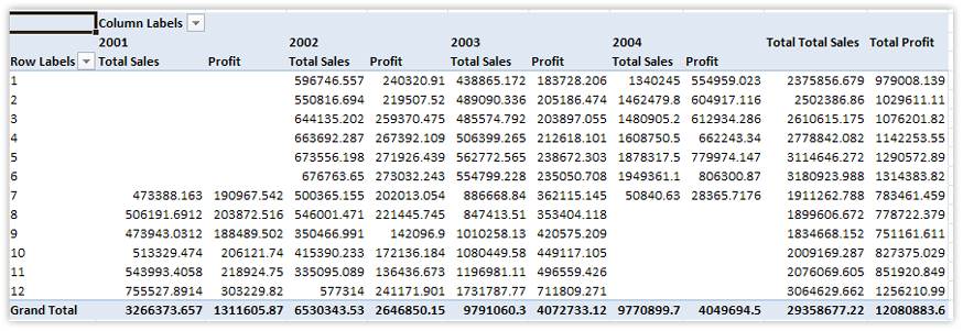
Figure 52 Profit measure added to pivot, along with Total Sales measure

Creating a Ratio Measure

OK, time for some fun. Here’s a new measure:

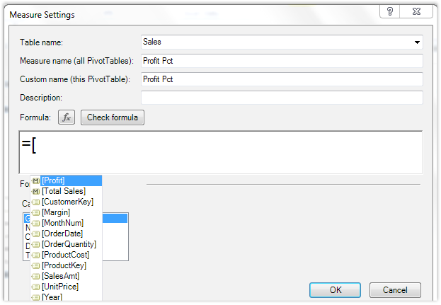
Figure 53 Adding a new measure, autocomplete triggered by “[“

Do you see the first item in the autocomplete list? Zooming in:

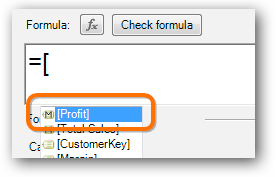
Figure 54 The [Profit] measure appears in autocomplete!

There’s even a little “M” icon, for measure, next to [Profit] in the autocomplete.

[Total Sales] is also in there, so let’s try:

=[Profit] / [Total Sales]

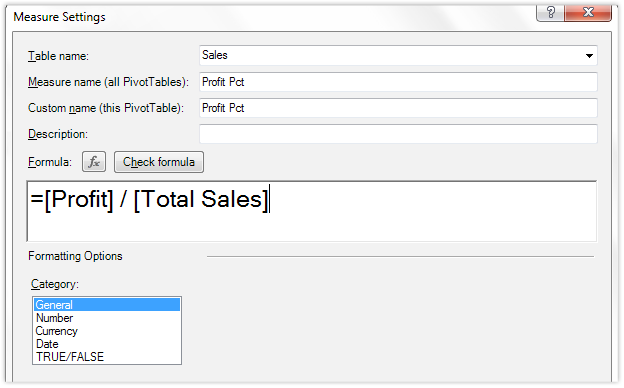
Figure 55 Measures can reference other measures, useful for creating things like ratios and percentages (and a million other things)

Original Measures do NOT Have to Remain on the Pivot

I’ll click OK now and create this new [Profit Pct] measure, but then I’ll uncheck the other two measures so we just see [Profit Pct] in the pivot:

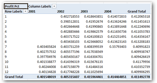
Figure 56 [Profit Pct] measure displayed by itself – its two “ancestor” measures are not required on the pivot

Changes to “Ancestor” Measures Flow Through to Dependent Measures

Let’s simplify the pivot a bit, and put the [Profit] measure back on:

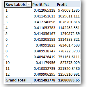
Figure 57 Removed [Year] from Columns, added [Profit] measure back

Let’s focus just on that first row for a moment:

Figure 58 About 41% for [Profit Pct], and 979k for [Profit]

What happens if we modify the formula for the [Profit] measure? Let’s find out.

Right click the [Profit] measure in the field list and choose Edit formula:

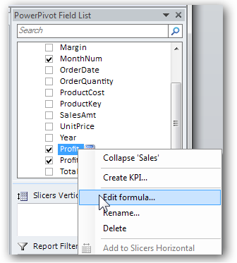
Figure 59 It is easy to open a measure to edit its formula

Now let’s do something silly. Let’s just arbitrarily boost our profits by 10%, by multiplying the original SUM formula by 1.1:

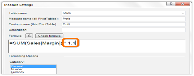
Figure 60 You would never do this in real life, unless you are, say, Enron

Click OK and let’s look at the first row in the pivot again:

Figure 61 [Profit] is now 10% higher, as expected. But that ALSO impacted [Profit Pct], since [Profit Pct] is based in part on [Profit].

Cases Where This Makes Real Sense

The model we’re working with here is pretty simple at the moment, and lacks things like Tax, Shipping, and Discount. It’s not hard to imagine defining [Profit] or [Total Sales] in ways that include/exclude those other miscellaneous amounts, and sometime later (perhaps much later) realizing that you need to change that.

In fact, it might just be a change in the business that triggers you to change your definition of [Total Sales] – it is not necessary that you made a mistake!

You may ultimately find yourself with literally dozens of measures (if not hundreds) that all depend back to more fundamental measures. Those dependencies can even run many “layers” thick – [X] depends on [Y] which depends on [Z] etc.

When you realize that you have hundreds of impacted calculations, but you only need to change a single formula to fix EVERYTHING, it is a glorious moment indeed.

It’s worth driving this point home, so I will restate it: Imagine having an entire suite of sophisticated Excel reports that all assume a certain calculation method for Profit and Sales. And then something fundamental changes, rendering that approach invalid. You could be performing spreadsheet surgery for days, perhaps weeks. If you use PowerPivot properly, that same situation might only take a few seconds to address.

The first time you experience this “I fix one thing and everything is updated” moment, you will know that your life has changed. How often do you find statements like that in a book about formulas? I’m guessing never, but it’s the truth :-)

Don’t “Redefine” Measures!

In order to reap the benefit outlined above, it’s important to use the names of measures in formulas rather than the formula that defined the original measure.

For instance, these two formulas for [Profit Pct] would return the same results:

=SUM(Sales[Margin]) / SUM(Sales[SalesAmt])

would yield the same results as:

=[Profit] / [Total Sales]

But only the second approach gives you the “fix once, benefit everywhere” payoff. So act accordingly.

Instinctively, I expected that tying everything tightly together like this, building “trees” of measures that depend on other measures, sometimes in layers, would lead to inflexibility and problems later on. In practice, that has never been the case. It has been all benefit in my experience.

Related: if you discover places where you need, for example, a Sales measure that is calculated differently, the right approach is just to define a second Sales measure with an appropriate name, such as [Sales – No Tax] or [Sales Incl Commissions], etc. That works splendidly. Seriously, I am smiling as I type this.

Other Fundamental Benefits of Measures

There are a few more benefits that no chapter titled “Intro to Measures” would be complete without. Let’s cover those quickly before continuing.

Use in Any Pivot

Up until now I have just been working with a single pivot. But if I create a brand-new pivot, guess what? All of the measures I created on that first pivot are still available in my new pivot!

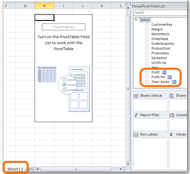
Figure 62 New pivot, new worksheet, but the measures are still available for re-use!

Centrally-defined Number Formatting

So far, I’ve been looking at ugly-formatted measures. Let’s add all three measures to this new pivot to illustrate:

Figure 63 Unformatted measures in my pivot

I can always use Format Cells, or even better, Number Format, to change this:

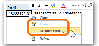
Figure 64 These two ways to format numbers in a pivot are SO antiquated! Be gone!

Instead, let’s bring up the measure editor for one of these measures:

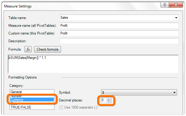
Figure 65 Setting [Profit] to be formatted as Currency, with 0 decimal places

The results are the same as if I had used Format Cells or Number Format:

Figure 66 [Profit] measure is now formatted nicely in the pivot, just as if I had used Format Cells or Number Format.

But that format now applies everywhere! Let’s return to my previous pivot and Refresh it:

Figure 67 I return to the first pivot, where [Profit] is still formatted “ugly,” and choose Refresh

The pivot picks up the new formatting!

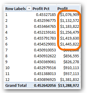
Figure 68 Currency formatting on [Profit] now shows up on original pivot, too

A refresh is not strictly required. Any manipulation of the other pivot will cause the formatting to be “picked up.” Reorder fields, click a slicer, click a “+” to drill down, etc. – all of these will cause the formatting to be picked up.

Now let’s set a percentage format on the [Profit Pct] measure:

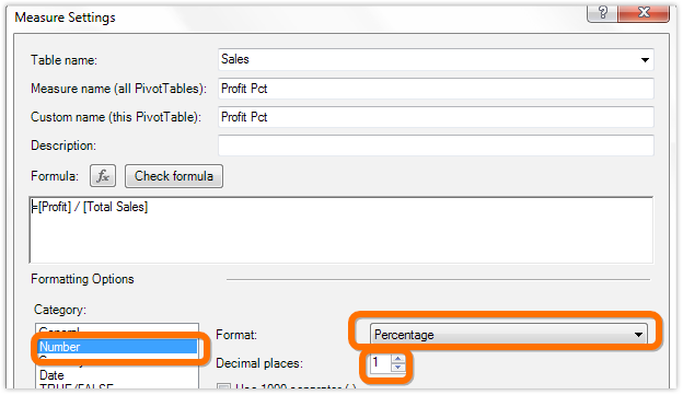
Figure 69 Formatting as Number, Percentage, 1 Decimal Place

The results are as expected:

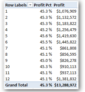
Figure 70 Percentage format? Check.

Whetting Your Appetite: COUNTROWS() and
DISTINCTCOUNT()

This chapter is running a bit long, but hey, there’s a lot of value to convey. And I still want to end with some “sizzle.”

Let’s use a couple of new functions to define two measures:

[Transactions] =

COUNTROWS(Sales)

and

[Days Selling] =

DISTINCTCOUNT(Sales[OrderDate])

When you see me use the syntax [Foo] = <formula>, that means I am creating a new measure named [Foo], with that formula. That way I don’t have to show screenshots of the Measure Editor every time I add a measure

Let’s see what that looks like:

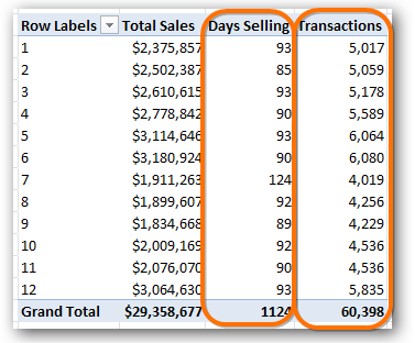
Figure 71 [Transactions] and [Days Selling] – introduction to COUNTROWS() and DISTINCTCOUNT()

COUNTROWS(Sales)

This function does exactly what it sounds like – it returns the number of rows in the table you specify. So for instance, in the figure above, there are 5,017 rows in the Sales table that have a MonthNum of 1.

I named this measure [Transactions] only because I know that each row in my Sales table is a transaction. But if a single transaction were spread across multiple rows, I couldn’t do that. I’d have to use COUNTDISTINCT() against a Transaction ID column, which I don’t have in this example.

DISTINCTCOUNT(Sales[OrderDate])

Again, this function does what it sounds like it does. It returns the number of distinct (unique) values of the column you specify.

So while there are 5,017 rows for MonthNum 1, and all of them obviously have a value for the [OrderDate] column, there are only 93 different unique values for [OrderDate] in those 5k rows.

Deriving More Useful Measures From These Two

Now I define two more measures that depend on the two measures above.

[Sales per Transaction] =

[Total Sales] / [Transactions]

and

[Sales per Day] =

[Total Sales] / [Days Selling]

Results:

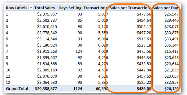
Figure 72 Two meaningful business measures – can’t do these in normal pivots!

Rearrange Pivot, Measures Automatically Adjust!

I remove MonthNum from Rows, drag ProductKey on instead, then drag Year to slicers and select 2002:

Figure 73 Completely scrambled the pivot, but my measure formulas still work!

Measures Are “Portable Formulas”

Stop and think about that “rearrange the pivot and the formulas still work” point for a moment. Let’s say your workgroup originally requested a report that displayed Sales per Day and Sales per Transaction, grouped by Month.

How would you build that report in normal Excel? You couldn’t just write formulas in a pivot. You’d have to do some pretty serious formula alchemy to get it working.

And those formulas, in normal Excel, would be very much “hardwired” to the “I want to see it by month” requirement.

Then some executive sees the report, loves it, and says “Wow, if only I could see this grouped by Product instead!”

Switching the normal Excel report over to be grouped by Product rather than Month (and sliceable by Year) would not be a modification. That would be starting from scratch, in many ways, and rebuilding the entire report.

With PowerPivot, you just drag fields around in the field list.

This is why I often describe measures as “portable formulas” – they can be used in many different contexts without needing to be rewritten. “Write once, use anywhere” is another way to say it. And even just the ability to re-use the same formula on another worksheet, in another pivot, by just clicking a checkbox, is a stunning example of portability. As your measure formulas become more sophisticated and powerful, this benefit becomes more and more impactful.

I even wrote a guest post for the official Excel blog on this topic, if you are interested:

http://ppvt.pro/PortableFormulas

But before we go any further, we need to talk about how measures actually work.