10- Thinking in Multiple Tables

A Simple and Welcome Change

In the opening chapters, I mentioned that PowerPivot offers a lot of benefits when you are working with multiple tables of data. But so far, I have shown none of those - I have only worked with the Sales table. Why have I waited?

Working with multiple tables is not complicated – it actually requires you to unlearn old habits more than it requires you to learn new ones. This is not going to be a difficult adjustment for you, just a little different.

The reason I waited until now to cover “multi table” is this: All of the concepts covered so far work the same way with multiple tables as they do with one table. I didn’t want to risk confusing you by teaching the CALCULATE() function at the same time as multi-table.

So this chapter really just extends what I have already covered, and shows how the same rules apply across tables as they do within tables.

Unlearning the “Thou Shalt Flatten” Commandment

Normal Excel literally requires that all of your data resides in a single table before you can build a pivot or chart against it. Since your data often arrives in multi-table format, Excel Pros have also become part-time Professional Data Flatteners.

• That usually means flattening via VLOOKUP(). Sometimes it means lots of VLOOKUP().

• Sometimes it involves database queries. Some Excel Pros who know their way around a database also write queries that flatten the data into one table before it’s ever imported.

You do not need to do either of these anymore. In fact, you should not.

In PowerPivot there are many advantages to leaving tables separate. It may be tempting to pull columns from Table B into Table A, especially using the new RELATED() function. You should resist this temptation. I sometimes use RELATED() to partially combine tables but only when debugging or inspecting my data. I delete that column when I am done with my investigation.

Got it? Just leave those tables alone. And if you already have flattened versions of your tables in your database, I actually recommend not using those versions – import the tables “raw” (separately).

Relationships Are Your Friends

This won’t be a step-by-step tutorial on the creation of relationships. I think that is well-covered in Bill’s book if you aren’t yet familiar with them.

But let’s create one very quickly. Take a look at my Products table:

Figure 118 I have not yet used the Products table, but it contains a lot of useful columns!

I’m going to create a relationship between Products and Sales, using the ProductKey column:

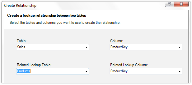
Figure 119 Relating Sales to Products

“Lookup” Tables

Note how I selected Products to be the Lookup table? That’s important. So important, in fact, that PowerPivot will not let me get it wrong. Let’s try reversing the two and see what happens:

Figure 120 I reversed Sales and Products, selecting Sales as my Lookup table, and I get a warning

Hover over the warning icon and I get an explanation:

Figure 121 PowerPivot detects that I got the order wrong, and when I click OK, Products will be correctly used as the Lookup table!

The use of the word “Lookup” was deliberate. Back at Microsoft, we chose that word so that it would “rhyme” with Excel Pros’ familiarity with VLOOKUP.

Think of Lookup tables as the tables from which you would have “fetched” values when writing a VLOOKUP. Lookup tables tend to be the places where friendly labels are stored for instance.

From here on, I will refer to the two tables’ roles in a relationship as the “lookup table” and the “data table.”

The Diagram View

This feature is new in PowerPivot v2, and it becomes very helpful as your models grow more sophisticated. But in smaller models, Diagram View is a fabulous gift to the authors of PowerPivot books, because we don’t have to spend long hours making graphical representations of tables and relationships :-)

Figure 122 The button for Diagram View is on the bottom-right corner of the PowerPivot window.

Clicking that button gives me:

Figure 123 Diagram View! All three tables displayed, with two of them linked by the relationship I just created.

Notice the direction of the arrow. The arrow always points to the Lookup table.

Using Related Tables in a Pivot

Now let’s revisit a pivot that uses ProductKey on Rows, and enhance it with some of the columns from this Products table.

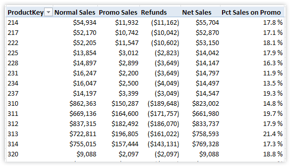
Figure 124 ProductKey pivot – but of course, ProductKey is meaningless to me.

OK, let’s remove ProductKey:

Figure 125 Be gone, ProductKey! And never show your face on a pivot again.

Now I’ll add ProductName from the Products table instead:

Figure 126 Checked the ProductName field in the field list, adding it to Rows

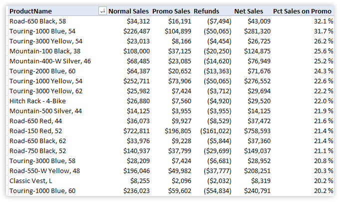
Figure 127 ProductName replaced ProductKey: much more readable

But I’m not limited to using any one field from Products – all of them can be used now that I have a relationship established. Let’s try a few different ones:

Figure 128 Category (from Products table) on Rows

Figure 129 SubCategory (also from Products table) nested under Category

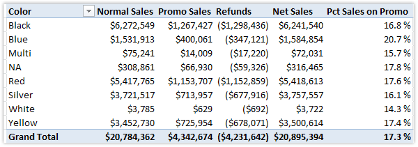
Figure 130 Even Color can be used! (Another column from Products table)

Why That Works: Filter Context “Travels” Across Relationships

Let’s examine a single measure cell and walk through the filter context “flow”:

Figure 131 Let’s examine how filter context flows for the highlighted measure cell

First, the Color=”Red” filter is applied to the Products table:

Figure 132 Products table filtered to Color=”Red” as result of filter context

The ProductKey column is not filtered directly, but it obviously has been reduced to a subset of its overall values, thanks to the Color=”Red” filter on the table.

Figure 133 Only those ProductKeys that correspond to Red products are left “active” at this point (63 ProductKey values out of a total of 397).

That filtered set of 63 ProductKeys then flows across the relationship and filters the Sales table to that same set of ProductKeys:

Figure 134 Sales table gets filtered (via relationship) to that same set of ProductKey values: {325; 324;…}

And then the arithmetic runs against the filtered Sales table. So it’s the same Golden Rules as before. Those rules just extend across relationships.

During the filter phase of measure evaluation, filters applied to a Lookup table (Products in this case) flow through to the Data table(s) related to that Lookup table.

This does NOT, however, apply in reverse: filters applied to Data tables don’t flow back “up” to Lookup tables.

Visualizing Filters Flowing “Downhill” – One of My Mental Tricks

In my head, I always see Lookup tables floating above the Data tables. That way the filters flowing “downhill” into the Data tables.

I’ll drag tables around in the Diagram View in order to represent that:

Figure 135 Products table dragged to be “above” Sales table

I also resized the tables so that the Data table (Sales) is bigger than the Lookup table (Products) – another mental trick.

I’ll now create a relationship from Customers to Sales. Here’s the updated diagram:

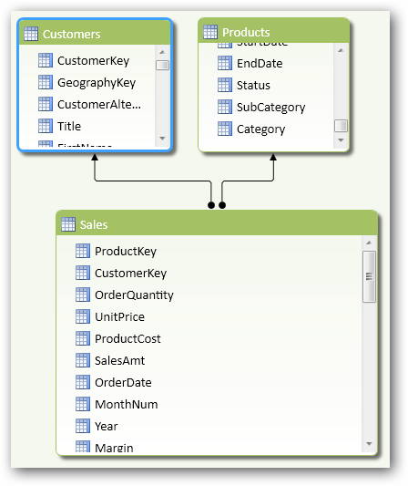
Figure 136 Two Lookup tables, both “above” the Data table that they filter

It’s a shame, in my opinion, that the relationship arrows flow toward the Lookup tables. Arrows point from Data to Lookup in the database world, but in PowerPivot I’d prefer that they point in the direction of filter flow. Yes, it’s the little things that bug me :-)

Filters from All Related Lookup Tables Are Applied

Let’s put columns from both Customers and Products on the same pivot:

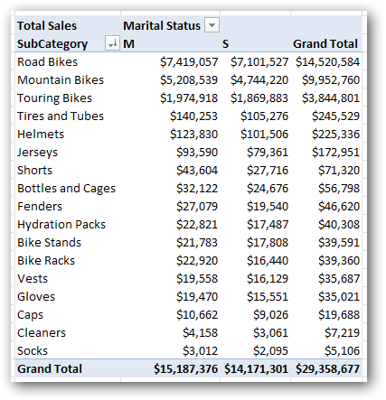
Figure 137 Products[SubCategory] and [Customers[MaritalStatus] on the same pivot: they each impact measures, as expected

This isn’t worth belaboring really – I just wanted to point out that you can use more than one Lookup table on a single pivot with no issue.

CALCULATE() <Filters> Also Flow Across Relationships

Until now, all of our <filter> arguments in CALCULATE have been filtering columns in the Sales table. But <filter> arguments are completely legal against Lookup tables (in fact, encouraged!), so let’s define a CALCULATE measure using a column in a Lookup table:

[Sales to Parents] =

CALCULATE([Total Sales], Customers[NumberChildrenAtHome]>0)

And compare that to its base measure, [Total Sales]:

Figure 138 Proof that CALCULATE <filters> also flow across relationships: [Sales to Parents] returns smaller numbers than its base measure [Total Sales]

I think that’s probably sufficient to explain the concept, but to be super precise, I should also say that <filters> in CALCULATE() are applied before filters flow across relationships.

Taking that precision one step further, here’s an updated version of the Filter Context Flow diagram:

Figure 139 Updated Filter Context flow diagram to highlight that relationship traversal happens after CALCULATE() <filters> are applied