16- SUMX() and Other X (“Iterator”) Functions

Need to Force Totals to Add Up “Correctly?”

Remember our [Sales per Day] measure? Let’s take another look at it:

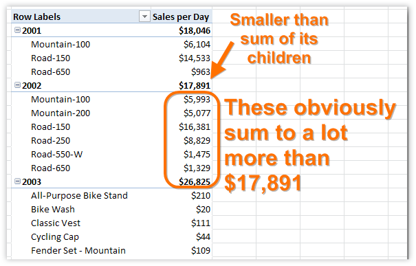
Figure 242 The subtotals do not match the sum of their parts

As your measures get more sophisticated, this will happen a lot: you will get subtotals and grand totals that don’t equal the sum (or even the average) of their children. (In this case, it’s because [Sales per Day] has a different denominator for each ModelName of bike).

Of course, many times that is 100% desirable. If you have an average temperature for each of the 12 months of the year, for instance, averaging those 12 numbers will not give you the average temperature for the year, since each month consists of a different number of days.

But again, in sophisticated measures (and business contexts) sometimes the correct logic for the smallest granularity is not correct for the next level up.

In other words, sometimes you need to force a total to equal the sum (or the average, etc.) of its children.

SUMX(), and other “X” functions like it, will help you do just that.

Anatomy of SUMX()

SUMX(<table or table expression>, <arithmetic expression>)

That’s it. Two arguments.

SUMX() operates as follows:

1. It steps through every single row in <table or table expression>, one at a time. You can pass a raw table name for this argument, or use a function that returns a table, such as VALUES() or FILTER(). The contents of <table or table expression> are subject to the filter context of the current measure cell. (This “stepping through” behavior is often described as “iterating.”)

2. For each row, it evaluates <arithmetic expression> using the filter context of the current row.

3. It remembers the result of <arithmetic expression> from each row, and when done, it adds them all up.

SUMX() in Action

Returning to the subtotals example, let’s look at the pivot again:

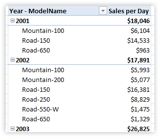
Figure 243 [Sales per Day] with Calendar[Year] and Products[ModelName] on Rows

Now we write a new measure:

[Sales per Day Totals Add Up] =

IF(HASONEVALUE(Products[ModelName]),
[Sales per Day],
SUMX(VALUES(Products[ModelName]), [Sales per Day])
)

So if we’re in the context of a single ModelName, it just uses the [Sales per Day] measure like the pivot already does. But when there is more than one ModelName, that means we’re in a total cell, and the SUMX() clause kicks in.

Note that I used VALUES(Products[ModelName]) for the <table or table expression> argument. That lets me be very specific – I want this SUMX() to step through all of the unique values of ModelName from the current filter context. If I specified the entire Products table instead (and no VALUES function), SUMX() would step through every row of the Products table from the current filter context, which might be a different number of rows.

Results:

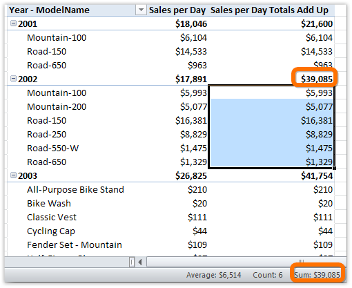
Figure 244 New measure: the totals are the sum of the individual models

Detailed Stepthrough

Just to drive it home, let’s walk through the evaluation of the SUMX() portion of the measure above, for the highlighted cell in the pivot:

Figure 245 We are going to step through how the SUMX() clause of the measure arrived at $21,600

Following the 3 points outlined in the “anatomy of SUMX()” section:

1. SUMX() steps through every row in VALUES(Products[ModelName]). The filter context provided by the pivot in this case is a completely unfiltered Products table because this cell is Year=2001, Products=All (it has no “coordinates” in the pivot from the Products table). So VALUES(Products[ModelName]) returns every single unique value of [ModelName] from the Products table.

How many values is that, actually? Let’s check.

[ModelName Values] =

COUNTROWS(VALUES(Products[ModelName]))

Figure 246 That is 119 values, even though we only see 3 on the pivot below 2001 in the prior screenshot!

Why 119 versus 3? All 119 are evaluated even in the original pivot, but because only 3 return non-blank results for [Sales per Day], that’s all the pivot showed us.

2. For each of those 119 values, SUMX() evaluates the [Sales per Day] measure. The Year=2001 filter context is maintained throughout this process, for every row. But the Products[ModelName] filter context changes every time SUMX() moves to the next of the 119 rows.

So it evaluates [Sales per Day] with filter context Year=2001, ModelName=”All-Purpose Bike Stand”, and that returns blank, because that model was not sold in 2001 (there are no rows in the Sales table with Year=2001, ModelName=”All-Purpose Bike Stand”.) Then it moves on to Year=2001, ModelName=”Bike Wash”, then Year=2001, ModelName=”Cable Lock”, etc.

Only three of those 119 rows in VALUES(Products[ModelName]) return non-blank results for [Sales per Day], and those are the three we saw displayed on the original pivot: “Mountain-100”, “Road-150”, and “Road-650”.

3. All 119 results of [Sales per Day] are then summed up. 116 blank values sum to 0 of course, and then the other three sum to $21,600.

MINX(), MAXX(), AVERAGEX()

These three operate in precisely the same manner as SUMX.

The only difference is in that last step – rather than summing up all of the results returned by each step, they then apply a different aggregation: MIN(), MAX(), or AVERAGE().

STDEVX.P(), STDEVX.S(), VARX.P(), VARX.S()

Again, these are exactly the same as all of the other “X” functions discussed so far, but I separated them out because of the “.P versus .S” flavors.

The difference between the P and S versions is precisely the same difference as that between the STDEVP() and STDEVS() functions in normal Excel. You use the P version when your data set represents the entire population of results, and the S function when all you have is a sample of the data.

It’s a statistics thing, not a DAX thing.

COUNTX() and COUNTAX()

Technically speaking, these are no different from the others mentioned so far. But there is a subtle difference when you think about it carefully.

Let’s return to our SUMX() example from before. Remember the formula? It was:

SUMX(VALUES(Products[ModelName]), [Sales per Day])

And it iterated through 119 unique values of ModelName, of which only 3 had non-blank values for [Sales per Day].

If we replaced SUMX() with COUNTX(), what would we get for an answer?

We’d get 3, because COUNTX() does not “count” blanks.

So we can think of COUNTX() as being “COUNT NONBLANK X()” really.

Why is This Different From COUNTROWS(), Then?

COUNTROWS() cannot take a measure as an argument, so it cannot be used to evaluate how many times that measure returns a non-blank value, which COUNTX() can do.

COUNTAX() versus COUNTX()

COUNTAX() also will also return 3 in this case, so it’s really no different in the vast majority of cases. There is one specific kind of case where COUNTAX() returns something different – I will use that as an example at the end of this chapter.

COUNTAX() treats the absence of rows, and blank results from a measure, exactly the same way as COUNTX(). The only place where COUNTAX() differs from COUNTX() is when you are counting text values in a column, and there are rows with text values of “” – rows that exist, but which contain an empty string. There will be an example of that at the end of this chapter.

Using the X Functions on Fields That Aren’t Displayed

In the one set of illustrations so far, you’ve seen SUMX() used to make totals add up “correctly.”

But you can also use an X function to loop over a field that is not on the pivot, then report back on what it found.

Let’s take the pivot we used for SUMX():

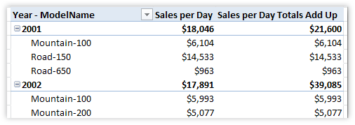
Figure 247 Where we left off with our completed SUMX() measure

And let’s add a new measure:

[Max Single-Country Sales] =

MAXX(VALUES(SalesTerritory[Country]), [Total Sales])

Results:

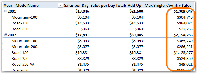
Figure 248 Interesting new measure, but is it correct?

Let’s check by adding Country to the pivot:

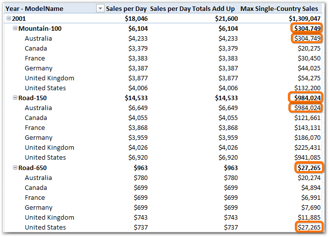
Figure 249 It is indeed reporting the max single-country sales

But Which Country?

Since this is most “magical” when the Country field is not on the pivot, one of the most common questions I get is “ok but how can I display which Country was the max when Country is not on the pivot? Knowing which one is just as important as knowing the amount.”

As of PowerPivot v2 there isn’t a function that just does that for you.

I did write a post on this though, that won’t fit here for space reasons. It uses the function FIRSTNONBLANK() – check it out here if you are interested: http://ppvt.pro/WhatDidXFind

RANKX()

OK, this one is actually quite a bit different from the others even though its syntax is similar.

Let’s do that whole “work backward from desired result” thing again:

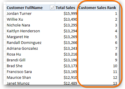
Figure 250 We want a measure that ranks customers by [Total Sales]

Here’s the formula for that rank measure:

[Customer Sales Rank] =

RANKX(ALL(Customers[FullName]), [Total Sales])

The Use of ALL()

The only difference we see so far is that I used ALL() instead of VALUES() in the first argument.

Why is that?

Because if I use VALUES(), I get 1’s for everyone:

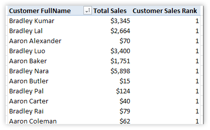
Figure 251 If I replace ALL() with VALUES(), everybody’s our #1 customer!

OK, why is that?

Well it makes some sense actually – for each row of the pivot, there is only one value of Customer[FullName] – so the RANKX measure ranks each customer as if he/she were the only customer in the world :-)

So by applying ALL(), I rank each customer against everyone else. I guess that’s intuitive, but the more I think about it, the more even that doesn’t feel right.

The pragmatic thing to do here is not worry about it. Just use ALL() and be happy we have the function :-)

Ties

Let’s look at the bottom of that same pivot, with ALL() restored so not everyone is #1:

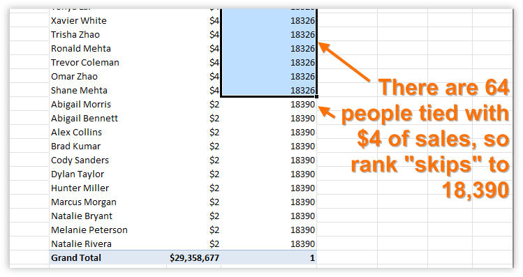
Figure 252 By default, ties are handled like this, but you can override that with the fifth (and optional argument), by setting it to Dense

The Optional Parameters

RANKX() actually has five parameters instead of the two possessed by the other X functions, but the last three are optional:

RANKX(<table or table expression>, <arithmetic expression>, <optional alternate arithmetic expression>, <optional sort order flag>, <optional tie-handling flag>

<optional alternate arithmetic expression> - The third argument to RANKX() may be the most mysterious thing in all of PowerPivot. If I weren’t writing this book, I would happily continue to ignore that I don’t understand it. I recommend always leaving it blank. Seriously. (But I will return to it in Chapter 17, because completely taking a “pass” on it doesn’t feel right).

<optional sort order flag> -This allows you to control rank order (ascending/descending) by setting to 1 or 0. It defaults to 0 if you leave it blank, which ranks largest values highest.

<optional tie-handling flag> - This can be set to Skip or Dense. It defaults to Skip, which is the behavior seen in the previous picture. If I change it to Dense, this is what the ties look at near the bottom of the pivot:

RANKX(ALL(Customers[FullName]), [Total Sales],,,Dense)

Figure 253 Dense tie handling – resumes with the very next integer after a series of tied ranks

Duplicate FullNames?

Very dangerous, this one. If you have two customers with the same FullName, they will be combined into a single customer and ranked unfairly high by their combined sales.

So make sure you rank by a unique field. I recommend concatenating CustomerKey or something unique with FullName so that you can still recognize the customer by name, and still maintain uniqueness.

I will be completely honest with you and say that as of PowerPivot v2, I don’t completely trust the RANKX() function yet. There are times when it does mysterious things – such as returning ties that I do not expect. I am not saying you shouldn’t use it, but that you should watch the results you get and make sure they meet your expectations before sharing. This may reflect the limits of my understanding of this function of course, in which case I think we need a version of RANKX() that is a bit more straightforward to use. I will update the blog if/when I hear something from my former colleagues at Microsoft.

Non-measure second arguments to the X functions. So far, I’ve only used measures for that second argument to these X functions.

But actually this is one place where you can break the “no naked columns” rule. You actually can just put a column name in for that second argument. And SUMX() will happily sum it.

In fact, you can even put a calculated column style formula in there, like Customers[YearlyIncome] / Customers[NumberOfChildren], and that will also work.

The COUNTAX() Mystery Solved!

The ability to use a non-measure expression as that final argument helps us solve the COUNTAX() conundrum.

When you use a measure as the second argument, I do not believe there is any situation in which COUNTX() and COUNTAX() will return different results.

But COUNTAX() will let you use a text column as the second argument, whereas COUNTX(), if you use a column as the second argument, requires that it be numeric or date type.

So here’s a silly little table I added to the PowerPivot window as a test:

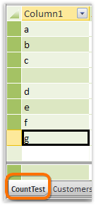
Figure 254 CountTest table – a testbed for COUNTAX()

Here’s a measure I wrote against it:

[COUNTAX Test] =

COUNTAX(CountTest, CountTest[Column1])

And the results:

Figure 255 The measure returns 7. From an 8-row table. So it didn’t count the one row with a blank value, which is different from the absence of a row. Subtle!

Change the COUNTAX() to COUNTX() and we get an error – COUNTX() refuses to accept a text column as the second argument.

So there you have it. The reason COUNTAX() exists.

(It’s actually more useful in calculated columns than measures, so this wasn’t really a “fair” test of its value).