20- Advanced Calculated Columns

Perspective: Calculated Columns Are Not DAX’s Strength

Let me be clear: I’m not saying that DAX is bad at calculated columns. I am just saying that measures are the magic in DAX, which is why I’ve spent the vast majority of the book on measures. I mean, we’ve always had calculated columns in Excel right?

OK, PowerPivot Calc Columns Are a Strength in Some Ways.

Well, even I have to stop for a moment and say: we’ve never had the ability to write a calc column against a 141 million row table now have we?

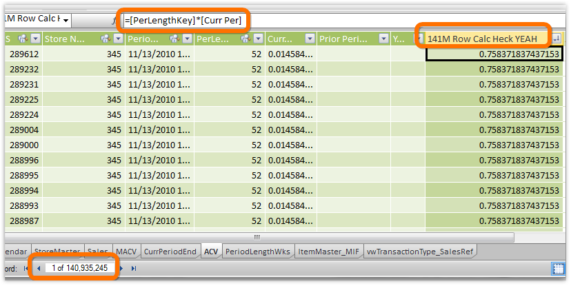
Figure 332 Calculated column written against a table with 141 million rows in it! (And this wasn’t some beast of a computer - I did this on my featherweight, 4 GB RAM Ultrabook that cost $899 retail in January 2012! Requires 64-bit of course.)

OK, so I’ll refine my point: other than the benefits provided by massive data capacity, seamless refresh, named reference, and relationships, PowerPivot calculated columns are nothing new to us :-)

But More Difficult in Some Cases

Actually, to be completely honest, PowerPivot calculated columns are actually a bit more difficult than normal Excel columns, at least in some circumstances, because PowerPivot lacks “A1” style reference.

In completely “row-wise” calcs, like [Column1] * [Column2], PowerPivot is no more difficult than normal Excel. But when you want to do something like “sum all the rows in this table where the [ProductID] is the same as this current row,” it gets a bit trickier.

I’m not criticizing PowerPivot for lacking A1-style reference. No, that was absolutely the correct decision. I just want to set your expectations – sometimes you will have to work a little harder in a PowerPivot calc column than you would in an Excel calc column, but even then, only when your calc goes beyond a single row.

Anyway, we’ll get to that. But first, some simple stuff that just didn’t fit anywhere else.

Start Out With “Not so Advanced”

OK, there are a couple of calculated column quick topics I’d like to cover that don’t really deserve the label “advanced” – they’re more “useful things I didn’t cover before because I was dying to get to measures.”

Grouping Columns

My favorite example of this is the Sales by Temperature, aka “Temperature Mashup” demo. In that demo, I import a table of temperature (weather) data, relate it to my Sales table, and then report [Sales per Day] broken out by temperature:

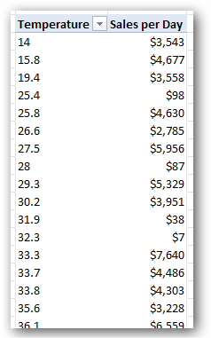
Figure 333 Sales per Day with Temperature on Rows, but the temperature is very precise

OK, I obviously do NOT care to see temperature ranges broken out by a tenth of a degree. I want to group them into more useful ranges.

You can do this with a calculated column. In the demo, here’s the formula I use in the Temperature table:

IF([Avg Temp]<40,"Cold",
IF([Avg Temp]<55,"Cool",
IF([Avg Temp]<70,"Warm",
"Hot"
)
)
)

Here’s what it looks like in the Temperature table as a calc column:

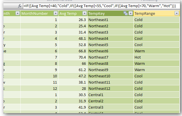
Figure 334 Grouping column in the Temperature table

And here’s what it looks like used on Rows instead of the Avg Temp column:

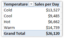
Figure 335 TempRange on Rows – MUCH better

I’ve used many kinds of formulas along these lines – ROUND() has been a very popular function for me in this regard, for instance.

To see the whole “Temperature Mashup” demo end to end that first debuted in 2009 (!), visit
http://ppvt.pro/TempMash

Unique Columns for Sorting

Did you notice that the sort order is “off” in that Temperature report? Here it is again:

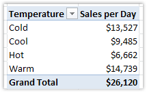
Figure 336 I would prefer the sort order to be Cold, Cool, Warm, Hot

OK, so let’s use the Sort by Column feature, and use AvgTemp to sort the TempRange column:

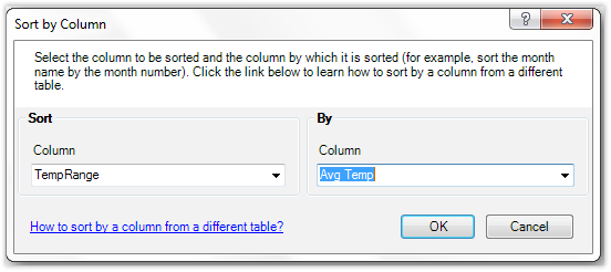
Figure 337 Attempting to use AvgTemp as the Sort By Column for TempRange

This yields an error:

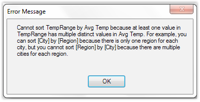
Figure 338 It does not like Green Eggs and Ham – not in a box, not with a fox. OK and it also doesn’t like AvgTemp as a Sort By Column.

I guess it could have used AvgTemp, since no single AvgTemp corresponds to two different TempRange values (48.1 for instance always maps to “Cool”), but PowerPivot doesn’t want to trust me. It wants each value of TempRange to have a single value in the Sort By Column, and as a former (and sometimes current) software engineer myself, I can understand why it doesn’t want to trust me :-)

So in this case, a SWITCH() does the trick –giving me a column with values 1-4:

SWITCH([TempRange], "Cold", 1, "Cool", 2, "Warm", 3, "Hot", 4)

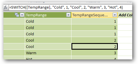
Figure 339 A valid candidate for a sorting column – this one works

Another Sort by Column Example

For a slightly more sophisticated problem, consider the “QtrYearLabel” column in my Periods table:

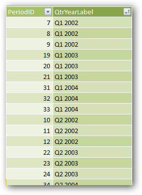
Figure 340 QtrYearLabel – note how each value matches multiple PeriodID values

I deliberately positioned it next to the PeriodID column so you could see that I have the same “matches multiple” problem here as what I had in the Temperature example.

But a SWITCH() isn’t going to save me this time. I need to do some math. Here’s a pattern that I use over and over again.

([Year] * 4) + [Qtr]

OK, in pattern form that is:

(<Year Column> * <number of periods per year>) + <period column>

Where “period” can be quarter (of which there are 4 per year), month (12), week (52), semester (2), whatever.

That gives me:

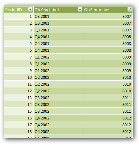
Figure 341 Unique sort id/sequence column for my QtrYearLabel column

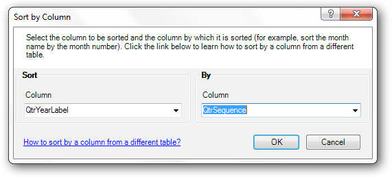
Figure 342 And this one works

Now For the Advanced Examples

Summing Up In a Lookup Table

Let’s say you wanted to create a Total Sales column in your Products table, reflecting the sales for each Product.

First, Rob would scold you. That’s what measures are for! Why would you summarize a value in your Lookup table? But then I would calm down and admit that there are definitely cases where you might occasionally need to do this :-)

It turns out that SUMX() can be used here, combined with the RELATEDTABLE() function:

SUMX(RELATEDTABLE(Sales), Sales[SalesAmt])

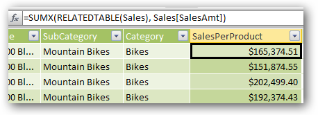
Figure 343 SUMX() – not just for measures anymore!

RELATEDTABLE() – you can think of this as a function that looks “backwards” across a relationship, from Lookup table to Data table, and returns all rows from the Data table corresponding to the current row in the Lookup table.

Note the use of a regular column reference for the second argument of SUMX(), which was something I introduced back in the chapter on the X functions. If you’re really curious as to why this all works, read the next section. If you’re just happy to have a pattern that works, just give it a skim.

Row Context – A Concept That’s Partly Critical but Mostly Ignorable :-)

The reason SUMX() allows a raw column reference in that second argument is that SUMX(), just like FILTER(), operates on a “one row at a time” basis when working its way through the rows in its first argument (the <table> argument). We’ve been talking a lot about filter context throughout the book, but technically there’s also another concept known as “row context.”

At a simple level, we can understand that a calc column implicitly calculates one row at a time. If I write a calc column formula like [PeriodId] + 1, the value of [PeriodId] from the current row is used to calculate each row of the new column. I mean, that’s just how calculated columns work. And that is the simplest example of row context.

I’m pretty sure that when you start writing more complex measures than those covered in this book, understanding row context as clearly as you understand filter context becomes important. But I’ve made it a long way without being able to expound in depth on the intricacies of row context in measures. Instead I say things like “FILTER() works one row at a time.” And row context just seems to make intuitive sense, most of the time, in calc columns.

So this little detour about row context is really an apology: when/if you discover that you really need to understand row context at that “next level,” I’m just not the guy to explain it to you. Or at least not yet. You can safely ignore it for now – I have for three years and am no worse for the wear, but guys like Marco Russo, Alberto Ferrari, and Chris Webb can do things in DAX that I can only copy. Go get one of their books if you outgrow what I have to teach you, and godspeed – think of me as a booster-phase rocket :-)

Simple Use of the EARLIER() Function

Ah, the EARLIER() function. It was two years before I understood how/when to use it, and even today, I admit that this function and I have only an uneasy peace. I’ve caught myself a few times using it when I didn’t actually have to, so mastery is still elusive.

That said, I am pretty confident in certain patterns for its use, and that’s really all you are going to need, at least for a long time.

Let’s extend the prior example from the Products table, and this time calculate a column that represents the total sales from all products with a matching Category.

In other words, you want something like this:

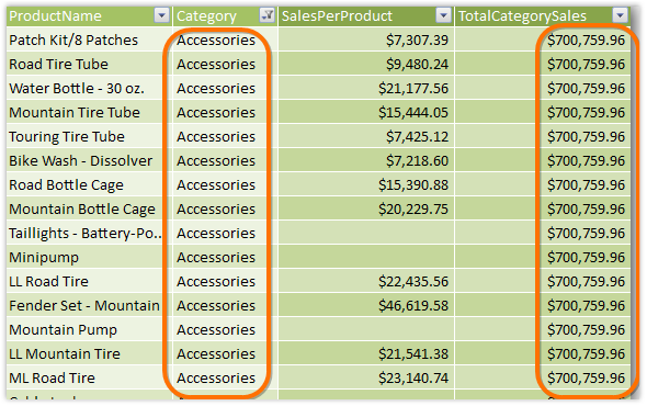
Figure 344 Every row with Category=Accessories sums to the same amount, which is the sum of all Accessories rows

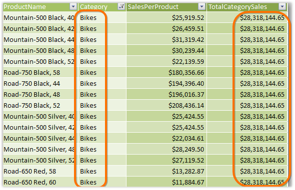
Figure 345 Filtered to Bikes

OK, here’s the formula:

CALCULATE(SUM(Products[SalesPerProduct]),
FILTER(ALL(Products),
Products[Category]=
EARLIER(Products[Category])
)
)

Whoa! CALCULATE() in a calc column! Yeah, things are getting crazy now :-) I have some explaining to do. I mean, this pattern looks a lot like the GFITW, but different. In fact, let’s think of it that way – we’re doing a “clear then re-filter,” just like in the GFITW. I can hear your questions now though…

• “Why no ALL(Products) outside the FILTER()?” – the last time we saw this sort of pattern, it was in the GFITW and it was in a measure. And there was an ALL() outside the FILTER() as well. So why not here? Well, in a calc column, there is no filter context. In other words, the filter context in a calc column is always set to ALL(), for everything! So we don’t need that ALL() outside the FILTER() – its role in the GFITW was to clear the existing filter context, which is already done for us in a calc column. (You can add an “outside” ALL here and it won’t impact your result).

• “OK then, why is the inside ALL() still there?” – you always ask the smartest questions! Well, inside a FILTER(), the notion of row context does exist. And we use the inside ALL() to get rid of our row context so that we’re looking at all rows in the table. Without the inside ALL(), our result for [TotalCategorySales] would be the same as [SalesPerProduct], which is not what we want.

• “Hmm, OK, I think I get that enough to at least use it. But what the heck is EARLIER()?” – this function basically says “hey you know that row context we’re using right now? I want to undo that, almost like hitting ctrl-Z, and go back to the previous row context we were using before.” Which is like a quantum physics explanation when all we really wanted to hear was “EARLIER() removes that inside ALL() we just applied so we can inspect the current row again.”

I really do think that all of this stuff could/should be made easier in a future version of PowerPivot. There should just be dedicated functions for these advanced calc column scenarios, named things like CALCSIMILARROWS() for this particular example. We don’t really need to understand these particular concepts as deeply as we understand the measure stuff, we just need them to work. And this FILTER() / EARLIER() stuff is really overkill – it forces us to get a bit “closer” to the DAX engine than we need to. Don’t feel bad if your head hurts a little right now. Just use the patterns here and don’t worry too much – it really is fine to do that. I have the credentials (or guts?) to call myself PowerPivotPro and yet that’s how I roll when it comes to advanced calc columns. You can too.

An Even More Advanced Example

I had to include this one, both because it shows a few twists on the previous technique, and because it is one of the coolest, most inspiring examples of the potential we all now have as Excel Pros.

I have a neighbor who’s a neuroscientist. In his field, he’s kind of a big deal, like Will Ferrell in the movie “Anchorman.” His name is Dan Wesson, he runs a research lab at Case Western Reserve University (CWRU), and his lab made it onto CNN earlier this year with some exciting developments in Alzheimer’s research. (See? People know him).

This is a well-funded lab with all kinds of expensive equipment. It’s an impressive place – I’ve toured it. He even has individual software packages that cost $10,000 for a single seat!

And oh yeah, with my help he’s converted most of his data analysis over to PowerPivot. You know, the next generation of spreadsheet. That thing that costs approximately $10,000 less than his other software. That’s right, Excel Pros – we even do Alzheimer’s research!

Here are a few of my favorite pictures of all time:

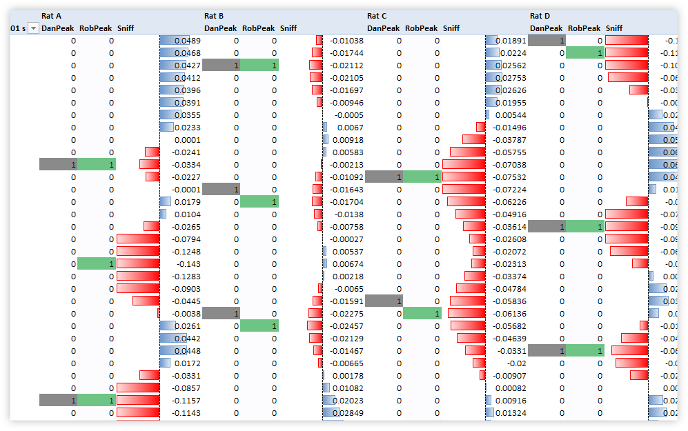
Figure 346 This “DNA” view is data from the Neuroscience lab at CWRU. The red and blue “waves” are rats inhaling and exhaling – red is inhale, blue is exhale, and each row represents 1/100 of a second!

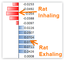
Figure 347 Zoomed in on one of the inhale/exhale waves.

Now here’s the one that makes me the happiest:

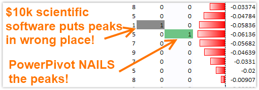
Figure 348 Detecting the peak of each inhale event is very important to Dan’s work. Look where the $10,000, purpose-built scientific software places the peaks versus where PowerPivot puts them!

That “peak detection” is just a calc column. Here’s what the data looks like:

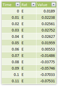
Figure 349 Time (in hundredths of a second), RatID, and Value - negative for inhale, positive for exhale. The bigger the absolute value, the more forceful the inhale/exhale.

The most critical component of detecting an inhale peak is finding the most negative value in any given timeframe. Think of it as like a moving average, except that it’s a moving minimum!

And here’s my calc column formula for moving minimum:

=CALCULATE(MIN(Data[value]),

FILTER(ALL(Data),

Data[Rat]=EARLIER(Data[Rat])

),

FILTER(ALL(Data),

Data[TimeID] <= EARLIER(Data[TimeID]) +5 &&

Data[TimeID] >= EARLIER(Data[TimeID]) –5

)

)

Hey, it’s still the same old “GFITW modified for calc column use,” just like the first example I showed you for the EARLIER() function. But there are a few wrinkles:

• Two FILTER() functions – don’t let this scare you. You can do as many as you want and the rules are still the same. A row has to “survive” both FILTER()’s in order to be eventually “fed” to the MIN() function that’s the first argument to the CALCULATE().

• The first FILTER() - is just like our previous example. Only rows for the current rat should be counted, otherwise we’re looking at someone else’s breathing :-)

• The Second FILTER() is kinda cool – it basically says “only count the five rows that happened sequentially before me, and the five rows that happened right after me.” So we end up looking at a window in time that is 11 rows “long,” which is actually 0.11 seconds.

The net result of the formula is that it tells us the smallest value in the current 11-row window.

From there, other calc columns can detect if the current row’s Value column matches the new 11-row minimum column, in which case we’re probably looking at a peak inhale.

See http://ppvt.pro/PkSniff for the full blog post, and see if you can spot the one mistake I made back then that I corrected in the formula above :-)

If you’re interested in reading more about this project, see:

http://ppvt.pro/Peak2Freq - where we move on to use our peak calc columns to produce frequency and amplitude measures.

http://ppvt.pro/FzzyTime - where we correlate the inhale/exhale data with events in another table that cannot be directly related (more calc column wizardry ensues)

There’s going to be another update on that project at some point, when Dan publishes the paper, so keep an eye on the Medical/Scientific category as well: http://ppvt.pro/MedSciCat

Memory and CPU Consumption of Complex Calc Columns

I think it’s appropriate to mention that certain kinds of calculated columns can eat a truly staggering amount of RAM when they’re running.

Take my “moving minimum” example from the peak detection scenario above for instance. That formula is written to only look at the previous five rows and the next five rows, plus the current row. So I’m only inspecting 11 rows at a time.

But to find those 11 rows to inspect, PowerPivot starts from scratch and goes looking through the entire table, one row at a time, and deciding whether each row belongs in that current window of 11.

In normal Excel, relative reference takes care of this – Excel literally goes and looks five rows up and five rows down. It does not have to scan the entire worksheet, row by row, in order to find the right 11 rows. When it comes to “look at the rows close to me,” PowerPivot is just fundamentally less intelligent than normal Excel. That’s a consequence of lacking A1-style reference, which I’ve said before is a necessary evil in order to get a truly robust environment.

I’ll leave you with one last observation on this topic: if you have one million rows in your table, that means scanning a million rows to calculate just a single row of the calc column. And since there are a million rows to calc, you have a million loops, each of which is a million rows of loop in itself. That’s literally a trillion comparisons! Not only does that take a lot of time and processor power, but it takes a lot of RAM too.

Ultimately, with Dan’s project, we had to abandon using PowerPivot calc columns for peak detection and implement the same “moving minimum” formula in SQL Server. That inhale/exhale table of his grew to be over 100 million rows! But we still use PowerPivot for all of the measures and reporting, which after all is PowerPivot’s strength.