Chapter 2
What is risk?

A main objective of a risk analysis is to describe risk. To understand what it means, we must know what risk is and how it is expressed. In this chapter, we define what we mean by risk in this book. We also look closer at the concept of vulnerability.

2.1 The risk concept and its description

We consider an activity, real or thought-constructed, for a specified period of time. The activity leads to some future consequences and these are not known—they are uncertain (). These two components, and , constitute risk:

The risk concept () covers (i) that the activity leads to some consequences , and (ii) that these consequences are not known ().

The consequences are with respect to something that humans value (health, the environment, assets, etc.). The consequences are often seen in relation to some reference values (planned values, objectives, etc.), and the focus is normally on negative, undesirable consequences. This definition does not, however, distinguish between positive and negative consequences (desirable and undesirable consequences), the point being that the activity results in some consequences (whatever they are). One possible restriction of this definition is introduced by requiring that there exists at least one outcome of judged as undesirable.

Often we split the consequences into events (for example, a disease, a gas leakage, a terrorist attack) and their consequences . Risk is then for short written (). The definitions () and () are equivalent. The shorter notation () does not represent any loss of generality as in () expresses all the consequences of the activity including the events .

As an illustration of the risk concept, think of a person's life where our focus is on his/her health condition. Now he/she is 40 years old. We are concerned about the health risk for this person for a specific period of time or the rest of his/her life. The consequences in this case relate to the occurrence or non-occurrence of specific diseases (known or unknown types) and other plagues, their time of occurrence and their consequences for the person (he/she may die, suffer, etc.). Following this definition, risk exists objectively in the sense of intersubjectivity. No one (with normal senses) would dispute that a human being can get some diseases and that we do not know in advance whether these diseases will occur or not. This definition of risk is general and also includes surprising events, for example, the person can get a new type of disease.

Thus, the risk concept has been defined. However, this concept does not give us a tool for assessing and managing risk. For this purpose, we must have a way of describing or measuring risk, and the issue is now how this should be done.

As we have seen, risk has two main dimensions—consequences and uncertainties–and a risk description is obtained by specifying the consequences and using a description (measure) of uncertainty, . The most common tool is probability (subjective probability or often also referred to as judgemental and knowledge-based probability), but others exist—see Section 2.4 and Aven et al. (2014). Specifying the consequences means to identify a set of quantities of interest that characterise the consequences , for example, the number of fatalities. The s are the high-level observable quantities of the risk analysis, such as profit, production, production loss, number of fatalities, number of attacks and the occurrence of an accident. These are the quantities that we should like to know the value of at the time of the decisions since they provide information about the performance of the alternatives studied. In the risk analysis, these quantities are predicted and the uncertainties assessed. We are performing the risk analysis to provide decision support for investment, design, operation and so on, and a set of decision alternatives are being considered.

Now, depending on the principles laid down for specifying and the choice of , we obtain different perspectives on how to describe/measure risk. As a general description of risk, we can write:

Risk description = (, (or alternatively, (, some specified events),

where is the background knowledge (models and data used, assumptions, etc.) on which and are based.

To simplify the presentation, we will normally just write and also when referring to specific s and s in the following. In the setting of a risk description, we always have in mind the specific and .

A common approach to risk assessment is to let , that is, knowledge-based probability is the tool used to express the uncertainties. However, this choice can be challenged; there is a need for seeing beyond the probabilities. We will return to this issue in Section 2.4. For now, unless otherwise stated, .

The probability is interpreted with reference to an uncertainty standard, for example, an urn (see Appendix A.1): if the assessor assigns a probability of an event A equal to say 0.1, it means that the assessor compares his/her uncertainty (degree of belief) about the occurrence of the event with drawing a specific ball at random from an urn that contains 10 balls. To show the dependency of the background knowledge that the probabilities are based on, we write . We may also use odds; if the probability of an event is 0.10, the odds against are 9:1. The assignments are based on available information and knowledge; if we had sufficient information, we would be able to predict with certainty the value of the quantities of interest. The quantities are unknown to us as we have lack of knowledge about how people would act, how machines would work and so on. Systems analysis and modelling would increase the background knowledge and thus hopefully reduce uncertainties. In some cases, however, the analysis and modelling could in fact increase our uncertainty about the future value of the unknown quantities. Think of a situation where the analyst is confident that a certain type of machine is to be used for future operation. A more detailed analysis may, however, reveal that also other machine types are being considered. And as a consequence, the analysts' uncertainty about the future performance of the system may increase. Normally, we would be far away from being able to see the future with certainty, but the principle is the important issue here; uncertainties related to the future observable quantities are epistemic, that is, they result from lack of knowledge.

Here are some more examples: the first one is linked to the health case introduced earlier.

Illness (Refer Figure 1.1)

Risk

: The occurrence or not of specific diseases (known or unknown types) and other plagues, their time of occurrence, and their consequences for a person (John) (he may die, suffer, etc.).

: Today we do not know if John will contract one or more of these illnesses, and we do not know what their consequences will be.

Risk description

: John contracts a certain illness next year.

: John's recovery time and overall health state, simplified in four categories: John recovers during the course of 1 month, 1 month 1 year, John never recovers, John dies as a result of the illness.

: Based on our knowledge of this illness , we can express a probability that John contracts this illness, for example, 10%, and that if he gets the illness, the probability that he will die is 5%. We write and . The symbol is read as ‘given’, so that expresses our probability that will occur given our knowledge .

: the knowledge on which these assessments are based on — referred to as the background knowledge (data, information, justified beliefs, assumptions)

Dose - response

Physicians often talk about the dose–response relationship. Formulae are established showing the link between a dose and the average response. The dose here means the amount of drugs introduced into the body, the training dose and so on. This is the initiating event . In most cases, it is known there is no uncertainty related to . The consequence (the response) of the dose is denoted . It can, for instance, be a clinical symptom or another physical or pathological reaction within the body. By establishing a dose–response curve, we can determine a typical (average) response value for a specific dose. In a particular case, the response is unknown. It is uncertain (). How likely it is that a specific will take different outcomes can be expressed by means of probabilities. These probabilities will be based on the available background knowledge . We may, for example, assign a probability of 10% that the response will be a factor 2 higher than the typical (average) response value.

Exposure - health effects

Within the discipline work environment, one often uses the terms ‘exposure’ and associated ‘health effects’. The exposure can, for example, be linked to biological factors (bacteria, viruses, fungi, etc.), noise and radiation. An initiating event could be that this exposure has reached a certain magnitude. The consequences the health effects are denoted , and we can repeat the presentation of the dose–response example.

Disconnection from server

Risk

: The occurrence or non-occurrence of a computer server failure and its consequences.

: Today we do not know whether the server will fail or not, and what the consequences will be in case of failures.

Risk description

: The computer server fails (no longer functions) over the next 24 hours.

: The effect on production, categorised as No consequences, reduced production speed and production stoppage.

: We know that the server has failed many times previously. Based on the historical data (), we assign a probability of 0.01 that the server will fail in the course of the next 24 hours. The failure of the server has never before led to a production shutdown. However, system experts assign a probability of 2% for a production shutdown in the event of a server failure. Hence, and .

: the background knowledge.

Fire in a road tunnel

Risk

: The occurrence or not of a fire in the tunnel and the consequences from such a fire.

: Today we do not know if there will be a fire in the tunnel and the consequences from such a fire.

Risk description

: A fire breaks out in a vehicle in a certain road tunnel during the next year.

: The losses of a fire, categorised as lightly injured road users, severely injured road users, killed, killed, more than 20 killed.

: We establish a model that expresses the relationship between the tunnel fire and various factors, such as traffic volume, traffic type and speed limit. We use the model in combination with historical data to assign a probability 0.1% that there will be a fire in the tunnel.

: the background knowledge.

Product sale

An enterprise that manufactures a particular product initiates a campaign toincrease sales.

Risk

: Sales (profitability)

: Today we do not know the sales and profitability numbers.

Risk description

: Sales quantity.

: Based on historical knowledge (), the probability that the sales will be less than 100 is expressed as .

: the background knowledge.

We may rephrase the above definition of risk by saying that risk associated with an activity is to be understood as (Aven and Renn 2009a):

Uncertainty about and severity of the consequences of an activity, where severity refers to intensity, size, extension, and so on, and is with respect to something that humans value (lives, the environment, money, etc). Losses and gains, for example, expressed by money or the number of fatalities, are ways of defining the severity of the consequences.

Hence, risk equals uncertainty about the consequences of an activity seen in relation to the severity of the consequences. Note that the uncertainties relate to the consequences ; the severity is just a way of characterising the consequences.

A low degree of uncertainty does not necessarily mean a low risk, or a high degree of uncertainty does not necessarily mean a high risk. Consider a case where only two outcomes are possible, 0 and 1, corresponding to 0 fatalities and 1 fatality, and the decision alternatives are and , having probability distributions (0.5, 0.5) and (0.0001, 0.9999), respectively. Hence, for alternative , there is a higher degree of uncertainty than for alternative . However, considering both dimensions, we would, of course, judge alternative to have the highest risk as the negative outcome 1 is nearly certain to occur.

If uncertainty is replaced by probability , we can define risk as follows:

Probabilities associated with the consequences of the activity, seen in relation to the severity of these consequences.

In the example above, (0.5, 0.5) and (0.0001, 0.9999) are the probabilities (probability distributions) related to the outcomes 0 and 1. Here, the outcome 1 means a high severity, and a judgement about the risk being high would give weight to the probability that the outcome will be 1.

However, in general, we cannot replace uncertainty by probability . This is an important point. The main argument is that probability is just a tool to express our uncertainty with respect to , and this tool is ‘imperfect’. We can have poor knowledge about a phenomena, but judge the probability of a related undesirable event to be small, say . Would we then give this probability much weight in a decision-making context? Probably not, as the knowledge supporting the probability is so weak. Uncertainties may in fact be hidden in the background knowledge, . For example, you may assign a probability of fatalities occurring on an offshore installation based on the assumption that the installation structure will withstand a certain accidental load. In real life, the structure could however fail at a lower load level. The probability did not reflect this uncertainty. Risk analyses are always based on a number of such assumptions.

The event in is referred to as a hazard or a threat. It is common to link hazards to accidental events (safety) and threats to intentional acts (security).

The event can also be associated with an opportunity. An example is a shutdown of a production system, which allows for preventive maintenance.

In a risk description we often add , a prediction of . By a prediction, we mean a forecast of which value this quantity will take in real life. In the product sale example, we would like to predict the sales. We may use one number, but often we specify a prediction interval such that will be in the interval with a certain probability (typical 90% or 95%). In the illness example, our focus will be on prediction of the consequence , given that the event has occurred, i.e., the time it takes to recover. Experience shows that on average it takes 1 month for recovery, and then we can use this as a prediction of the consequence .

Using a number such as this is problematic, however, as the uncertainty about the consequence is often large. It is more informative to use a prediction interval or formulate probabilities for various consequence categories of , for example: the person will recover within 10 days, the person will recover within 1 month, the person will never recover or the person will die. We will return to such descriptions in Section 2.3.

2.2 Vulnerability

A concept closely related to risk is vulnerability. It is basically risk conditional on the occurrence of an event .

Let us return to the illness example in Chapter 1. If the person (John) contracts the illness, that is, occurs, what will be the consequences then? It depends on how vulnerable he is. He may be young, old, physically strong or already weakened before contracting the illness. We use the concept vulnerability when we are concerned about the consequences, given that an event (in this case, the illness) has occurred. As mentioned earlier, we often refer to this event as an initiating event. Looking into the future, the consequences are not known, and vulnerability is then to be understood as the combination of consequences and the associated uncertainty, that is, , using the notation introduced earlier.

The vulnerability description takes the general form (, given .

When we say that a system is vulnerable, we mean that the vulnerability is considered to be high.

If we know that the person is already in a weakened state of health prior to the illness, we can say that the vulnerability is high. There is a high probability that the patient will die.

Vulnerability is an aspect of risk. Because of this, the vulnerability analysis is a part of the risk analysis. If vulnerability is highlighted in the analysis, we often talk about risk and vulnerability analyses.

2.3 How to describe risk quantitatively

As explained earlier, a description of risk contains the following components (). How are these quantities described? We have already provided a number of examples of how we express , but here we will take a step further. We consider two areas of application, economics and safety. But first we recall the definition of the expected value, , of an unknown quantity, , for example, expressing costs or the number of fatalities. Here is an example of using the above terminology. If can assume three values, say and , with respective probabilities of 0.1, 0.6 and 0.3, then the expected value of is

We interpret as the centre of gravity of the probability distribution for . See Appendix A.1.

Imagine a situation where we are faced with two possible initiating events and , for example, two illnesses. Should these events occur, we would expect consequences and , respectively. If we compare these expected values with the probabilities for and , we obtain a simple way of expressing the risk, as shown in Figure 2.1. If the event's position (marked *) is located in the far right of the figure, the risk is considered high, and if the event is located in the far left, the risk as described by these dimensions is low.

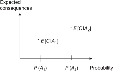
Figure 2.1 Risk description for two events and , with associated expectations and .

An alternative risk description is obtained by focusing on the possible consequences or consequence categories, instead of the expected consequences. We return to the illness example, where we defined the following consequence categories:

: The person recovers in 1 month

: The person recovers in 1 month 1 year

: The person never recovers

: The person dies as a result of the illness

For illness , we can then establish a description as shown in Figure 2.2. Here expresses the probability that the person contracts the actual illness and recovers within 1 month, that is, 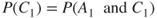. We interpret the other probabilities in a similar manner.

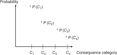
Figure 2.2 Risk description based on four consequence categories.

Alternatively, we may assume that the analysis is carried out conditional on the event that the person is already ill, and then expresses the probability that the person will recover in a month. In this case, is to be read as .

It is common to use categories also for the probability dimension, and the risk description of Figure 2.2 can alternatively be presented as in Figure 2.3. We refer to the figure (matrix) as a risk matri2. We see that the use of such matrices could make it difficult to distinguish between various risks since it is based on rather crude categories.

Consequences
Probability
Highly probable
Higher than 50%	x
Probable
		x
Low probability
			x	x
Unlikely
Less than 2%

Figure 2.3 Example of a risk matri2. The in column shows that there is a probability greater than 0.5 for consequence . The numbers are conditional that the person is ill.

Often a logarithmic or an approximately logarithmic scale is used on the probability axis. Risk matrices can be set up for different attributes, for example, with respect to economic quantities and loss of lives. We present a number of examples of risk matrices throughout the book. We also provide an in-depth discussion of the method. The reader is referred to Section 13.3.2.

2.3.1 Description of risk in a financial context

An enterprise is considering making an investment, and we denote the value of the return on this investment next year by . Since is unknown, we are led to predictions of and uncertainty assessments (using probabilities). Instead of expressing the entire probability distribution of , it is common to use a measure of central tendency, normally the expectation, together with a measure of variation/volatility, normally taken as the variance, standard deviation or a quantile of the distribution, for example, the 90% quantile , which is defined by .

Based on average returns in the market for this type of investments, the enterprise establishes an expectation (prediction). However, the actual value may show a significant deviation from this value, and it is the deviation that one is especially concerned about in this context. Risk and the risk analysis have their focus on the uncertainties viewed in relation to the market average values. The variance and the quantiles thus become important expressions of risk. In the economic literature, the concept ‘Value-at-Risk’ (VaR) is often used for such a quantile. A VaR with a confidence of 90% is equal to the 90% quantile .

2.3.2 Description of risk in a safety context

In a safety context, terms such as ‘FAR’, ‘PLL’, ‘IR’, and ‘F-N-curve’ are commonly used. We will explain these terms below.

In situations where risk is focused on loss of lives, the FAR (Fatal Accident Rate) value is often used to describe the level of risk.

The FAR value is defined as the expected loss of life per 100 million () hours of exposure.

When the FAR concept was introduced, hours corresponded to the time of 1000 persons present at their workplace through a full life span. Today it takes 1400 persons to reach 100 million working hours. The FAR value is often related to various categories of activities or personnel. Such activity- or personnel-related FAR values are usually more informative than average values.

The expected number of fatalities over a year is referred to as PLL (Potential Loss of Life).

If we assume that there are persons exposed to a risk for hours per year, the connection between PLL and FAR can be expressed by the following formula:

The average probability of dying in an accident for persons, referred to as the AIR (Average Individual Risk), can be expressed as

Another form of risk description is associated with the so-called safety functions. Examples of such functions are

• preventing escalation of accident situations so that personnel outside the immediate accident area are not injured;
• maintaining the capacity of main load-bearing structures until the facility has been evacuated;
• protecting rooms of significance to combatting accidents so that they remain operative until the facility has been evacuated;
• protecting the facility's safe areas so that they remain intact until the facility has been evacuated;
• maintaining at least one escape route from every area where personnel are found until evacuation to the facility's safe areas and rescue of personnel have been completed.

Risk associated with loss of a safety function is expressed by the probability, or the frequency, of events in which this safety function is impaired. This form of risk description has its origin in analysis of offshore installations and is especially useful in the design phase.

In many cases, crude categories are used for both probability and consequences, as illustrated in the risk matrix (Figure 2.4).

Consequences	Insigni-	Small	Moderate	Large	Very large
	ficant	Non-serious	Serious	Serious injuries	More than
		injuries	injuries	fatalities	2 fatalities
Probability
Highly probable
Less than 1 year
Probable
years
Low probability
years
Unlikely
50 years or more

Figure 2.4 Example of a risk matri2. The category ‘Unlikely’ corresponds to a prediction of one event in 50 years or more, ‘Low probability’ corresponds to a prediction of one event in 10–50 years and so on.

An alternative categorisation based on probability for a given year is shown in Figure 2.3.

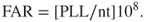
An F–N curve (Frequency–Number of Fatalities) is an alternative way of describing the risk associated with loss of lives; refer to Figure 2.5. An F–N curve shows the frequency of accident events with at least fatalities, where the axes are normally logarithmic. The F–N curve describes the risk related to large-scale accidents and is thus especially suited for characterising societal risk.

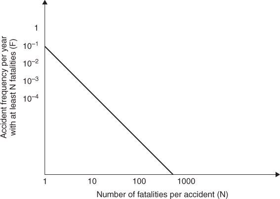
Figure 2.5 Example of an F–N curve (Frequency–Number of fatalities).

In a similar way, accident frequencies for personal injuries, environmental spills, loss of material goods and so on can be defined.

Note that frequency is an average number of events per unit of time or per operation. The connection between frequency and probability is illustrated by the following example. Assume that for a specific company we have calculated the frequency of accidents leading to personnel injuries, at 7 per year, that is, 7/8760 = 0.0008 per hour. From this rate, we may assign a probability of 0.0008 that such an accident will occur during 1 hour. This approach for transforming frequencies to probabilities works when this value is small—how small depends on the desired accuracy. As a rule of thumb, one often uses ‘less than 0.10’.

It is also common to talk about observed (historical) PLL (number of fatalities per year) values, FAR (the number of fatalities per 100 million exposure hours) values and so on.

Various normalisations may be used depending on the application involved. For example, in a vehicular transport context, we are primarily concerned with the (expected) number of fatalities and injuries per kilometre and year.

2.4 Qualitative judgements

First let us again reflect on why we need to see beyond probability to express risk. A probability expresses the degree of belief concerning the occurrence of an event given some background knowledge. Suppose that a probability equal to 0.5 is assigned in a particular case. This value can be based on strong or weak background knowledge, in the sense that in one case there is a significant amount of relevant data and/or other information and knowledge that supports a value of 0.50, while, in another case, few or no data or other information/knowledge support this value. Let us look at an extreme case. You hold a normal coin and throw it. You specify a probability of 0.50 for observing a head—the background knowledge is strong. The probability judgement is based on the argument that both sides are equally likely because of symmetry, and experience of such coins supports getting a head in roughly 50% of throws. But let us imagine that you are to assign the probability of a new coin that you know nothing about, it can be normal or abnormal (you will not see it). What is then your probability? You will most probably still say 50%. But now the background knowledge is weak. You have little insight into what kind of coin this is. We see that we get the same probability, but the background knowledge in the former case is strong and weak in the latter case. When assessing the ‘strength’ of an assigned probability, it is clearly important to also consider the background knowledge. The number alone does not say much. This is the situation when we use probabilities to describe the risk. The figures are based on background knowledge, and we must some know how strong this is to use the numbers in the right way in the risk management. The following aspects have to be considered: How good are the data and models that support the probability judgements? What about the expert opinions included? And all the assumptions made—how reasonable are they?

Hence, standard risk matrices must be used with care. We must be aware that they have clear limitations in terms of providing a picture of the risk associated with an activity and that one cannot use them to draw conclusions about what is acceptable risk and what is not. For an assignment of the probability and consequences of an event, the strength of the underlying knowledge could be strong or weak, but it is not possible to see this from the probability figures alone. One can conveniently highlight the events where the background knowledge is relatively weak, so that one is particularly careful to draw conclusions on the basis of probability assignments of such events. See the illustration in Figure 2.6.

Consequences	Insigi-	Small	Moderate	Large	Very large
	ficant	(Non-	(Serious	(Serious	(>2 fatalities)
		serious	injuries)	injuries
Probability		injuries)		fatalities)
Highly probable
(<1 year)
Probable
( years)		•
Low probability
( years)
Unlikely
(50 years or more)

Figure 2.6 Example of a risk matrix, where the assignments are supported by strong, medium and weak background knowledge. Strong knowledge: •, medium strong knowledge: : and weak knowledge: .

To assess this strength, a score system with three categories as suggested by Flage and Aven (2009) could, for example, be used:

The knowledge is weak if one or more of these conditions are true:

• The assumptions made represent strong simplifications.
• Data/information are non-existent or highly unreliable/irrelevant.
• There is strong disagreement among experts.
• The phenomena involved are poorly understood, models are non-existent or known/believed to give poor predictions.

If, on the other hand, all (whenever they are relevant) of the following conditions are met, the knowledge is considered strong:

1. 1. The assumptions made are seen as very reasonable.
2. 2. Large amount of reliable and relevant data/information are available.
3. 3. There is a broad agreement among experts.
4. 4. The phenomena involved are well understood; the models used are known to give predictions with the required accuracy.

Cases in between are classified as having a medium strength of knowledge.

A simplified version of these criteria is obtained by using the same score for strong but give the medium and weak scores for a suitable number of conditions not met, for example, medium if one or two of the conditions 1–4 are not met and the is score weak otherwise, that is, when three or four of the conditions are not met.

The strength illustrated in the risk matrix could be shown by coloured events, for example, red (dark), yellow (dashed) or green (light), depending on whether the background knowledge is considered to be weak, medium or strong, respectively, or as illustrated in Figure 2.6: Strong knowledge: •; medium strong knowledge: and weak knowledge: .

An alternative approach is presented by Aven (2013d) for assessing the strength of knowledge of , by assessing the risk associated with deviations from the assumptions made (assumption deviation risk).

The quantitative analysis can be supplemented in many other ways, for example, by introducing a red team (devil's advocate) addressing issues such as the following:

• Searching for unknown knowns, that is, events that are known by others, but not by the original analysis group
• Arguing for the occurrence of events that are considered to have negligible probability
• Checking that relevant signals and warnings have been properly reflected.

The point is to challenge the judgements and assumptions made in the quantitative analysis.